The Hidden Math Behind Precision: How to Calculate Standard Error
Standard error is the silent architect of statistical confidence. It quantifies the uncertainty inherent in sample-based estimates, transforming raw data into actionable insights. Without it, researchers would navigate blindly—assuming precision where variability lurks. Yet, few grasp the exact mechanics of how to calculate standard error, let alone its nuanced applications across fields from clinical trials to market forecasting. The formula itself—simple on paper, complex in practice—demands more than rote memorization. It requires an understanding of sampling distributions, variance, and the delicate balance between bias and efficiency.
The misconception persists that standard error is merely an academic abstraction. In truth, it is the bridge between theory and real-world decision-making. A pharmaceutical company testing a new drug relies on it to determine dosing confidence. A pollster predicting election outcomes uses it to frame margin-of-error claims. Even machine learning models, where overfitting is a constant threat, depend on standard error to validate generalization. Yet, the path from sample data to a reliable standard error estimate is fraught with pitfalls—from incorrect assumptions about population distribution to mishandling small sample sizes. Mastery here isn’t optional; it’s a prerequisite for credible analysis.
The Complete Overview of How to Calculate Standard Error
At its core, how to calculate standard error hinges on two pillars: the standard deviation of the sample and the sample size. The standard error (SE) of a statistic—most commonly the mean—is derived by dividing the sample’s standard deviation by the square root of its count. This adjustment accounts for the fact that larger samples yield more stable estimates, reducing the "noise" introduced by random sampling fluctuations. However, the process extends beyond this basic formula. For proportions, the calculation differs, incorporating the binomial distribution’s inherent variability. What remains constant is the principle: standard error measures how far sample statistics might deviate from the true population parameter, on average.The complexity arises when real-world data defies ideal assumptions. Non-normal distributions, heteroscedasticity (unequal variances), or autocorrelated observations (common in time-series data) can distort standard error estimates if ignored. Researchers must then employ robust alternatives—bootstrapping, jackknifing, or finite-population corrections—to ensure accuracy. The choice of method isn’t arbitrary; it depends on the data’s structure and the analysis’s goals. For instance, a clinical study with skewed treatment responses may require a non-parametric approach, while a survey of voter preferences might rely on asymptotic approximations. Understanding how to calculate standard error thus demands flexibility, not dogma.
Historical Background and Evolution
The concept of standard error emerged from the 19th-century statistical revolution, when mathematicians sought to quantify the reliability of empirical observations. Karl Pearson’s 1894 work on correlation laid early groundwork, but it was Ronald Fisher in the 1920s who formalized the distinction between sample and population parameters. Fisher’s introduction of the standard error of the mean (SEM) provided a framework to assess sampling error, linking probability theory to practical inference. His innovations—including the t-distribution for small samples—were pivotal, as they addressed the limitations of earlier normal-distribution assumptions.The evolution continued with Jerome Cornfield and others refining how to calculate standard error for proportions in the mid-20th century, adapting binomial theory for survey research. Computational advances in the 1980s further democratized these techniques, as software like SAS and R automated once-laborious calculations. Today, the field has splintered into specialized branches: from Bayesian approaches that incorporate prior distributions to machine learning’s reliance on standard errors for model evaluation. Yet, the foundational principles remain unchanged—standard error is still the compass guiding researchers from uncertainty to insight.
Core Mechanisms: How It Works
The mechanics of how to calculate standard error begin with the sample standard deviation (s), a measure of data dispersion. For a mean, the formula is:SE = s / √n where n is the sample size. This reflects the Central Limit Theorem’s assertion that sample means cluster around the population mean with a spread proportional to 1/√n. For proportions (p̂), the formula adjusts to:
SE = √[p̂(1−p̂)/n] Here, the binomial variance (p̂(1−p̂)) accounts for the binary nature of categorical data.
The subtlety lies in recognizing when to use these formulas—and when to deviate. For instance, if the sample is drawn without replacement from a finite population (e.g., a company’s 500 employees), the finite population correction factor (FPC) modifies the denominator to:
SE = s / √[n(1 − (n/N))]
where N is the population size. This adjustment prevents overconfidence in small samples relative to the whole. The choice of method isn’t just mathematical; it’s a judgment call about the data’s context.
Key Benefits and Crucial Impact
Standard error is the unsung hero of statistical rigor. It transforms raw estimates into credible intervals, allowing researchers to state not just what a sample suggests but how confidently. In medicine, this means distinguishing between a drug’s true efficacy and placebo-like variability. In economics, it clarifies whether a reported GDP growth rate is statistically significant or merely noise. The impact extends to everyday decisions: a poll’s ±3% margin of error is standard error in action, translating uncertainty into public trust.Table of Contents
- The Complete Overview of How to Calculate Standard Error
- Historical Background and Evolution
- Core Mechanisms: How It Works
- Key Benefits and Crucial Impact
- Major Advantages
- Comparative Analysis
- Future Trends and Innovations
- Conclusion
- Comprehensive FAQs
- Q: Can I calculate standard error for a median instead of a mean?
- Q: How does standard error relate to confidence intervals?
- Q: What’s the difference between standard error and standard deviation?
- Q: Are there scenarios where standard error isn’t reliable?
- Q: How can I reduce the standard error of my estimates?
- Q: Can standard error be negative?
- Q: How do I calculate standard error for a regression coefficient?
The stakes are highest where miscalculation has consequences. A 2012 study in Nature revealed that over half of published research in top psychology journals contained errors—many traceable to improper standard error handling. The issue isn’t ignorance but the complexity of how to calculate standard error under non-ideal conditions. When distributions are skewed, when samples are clustered, or when missing data introduces bias, standard error becomes a moving target. Yet, the alternative—ignoring it—risks flawed conclusions with real-world repercussions.
"Standard error is the price we pay for looking at the world through a sample rather than the whole. The art lies in paying it wisely." — Nassim Nicholas Taleb, Antifragile
Major Advantages
- Precision in Estimation: Standard error quantifies the "error bar" around sample statistics, enabling honest communication of uncertainty. For example, a mean income estimate of $50,000 with an SE of $1,000 implies a tighter confidence than the same mean with an SE of $5,000.
- Hypothesis Testing: It underpins t-tests, z-tests, and ANOVA by defining critical values for significance. Without SE, p-values would lack context, leading to false positives or negatives.
- Sample Size Planning: Researchers use SE to determine how large a study must be to achieve a desired margin of error, balancing cost and reliability.
- Model Validation: In regression analysis, standard errors of coefficients assess their stability. High SE suggests the model may overfit or omit key variables.
- Risk Assessment: Industries from finance to healthcare use SE to stress-test predictions, identifying where variability could lead to catastrophic outcomes.

Comparative Analysis
| Standard Error of the Mean (SEM) | Standard Error of the Proportion (SEP) |
|---|---|
|
|
Future Trends and Innovations
The future of how to calculate standard error lies in hybrid approaches that marry classical statistics with machine learning. Bayesian methods, which treat parameters as distributions rather than fixed values, are gaining traction for their ability to incorporate prior knowledge—critical in fields like genomics where data is scarce. Meanwhile, deep learning models are being retrofitted with uncertainty quantification tools, using standard error-like metrics to flag unreliable predictions. The challenge remains computational: as datasets grow, traditional SE calculations become prohibitively slow, necessitating approximations or sampling-based alternatives like Monte Carlo simulations.Another frontier is adaptive standard errors, where the calculation dynamically adjusts to data patterns. For example, in time-series analysis, heteroscedasticity-consistent SEs (HAC) account for changing variance over time. As automation tools like Python’s `statsmodels` or R’s `lme4` package democratize these techniques, the risk of misuse rises. The next decade may see a shift toward "statistical literacy" as a prerequisite for data science roles, ensuring that how to calculate standard error isn’t just a technical skill but a philosophical guardrail against overconfidence.

Conclusion
Standard error is more than a formula; it’s a lens through which to view data’s inherent limitations. The process of how to calculate standard error forces researchers to confront the gap between sample and population, between observation and truth. In an era of big data, the temptation to ignore uncertainty is strong—but the cost of doing so is measured in wasted resources, misleading policies, and eroded trust. The tools exist to compute SE accurately, from basic calculus to advanced bootstrapping. What’s needed now is a cultural shift: treating standard error not as an afterthought but as the foundation upon which all inference stands.The math itself is straightforward. The art lies in applying it wisely—knowing when to trust the formula, when to question its assumptions, and when to seek alternative methods. As data grows more complex, the principles remain: precision demands humility, and standard error is the measure of both.
Comprehensive FAQs
Q: Can I calculate standard error for a median instead of a mean?
A: Yes, but the method differs. For medians, especially with small or skewed samples, bootstrapping is often used to estimate the standard error by resampling the data and calculating the median’s variability across resamples. Traditional formulas (like SEM) assume normality and are inappropriate for medians.
Q: How does standard error relate to confidence intervals?
A: Standard error directly determines the width of confidence intervals. For a 95% CI around a mean, the interval is calculated as mean ± (1.96 × SE). A smaller SE yields narrower intervals, indicating higher precision in the estimate. The relationship is inverse: reducing SE (via larger samples or lower variance) tightens the CI.
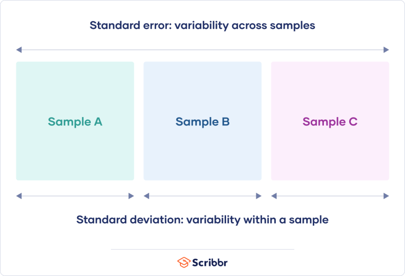
Q: What’s the difference between standard error and standard deviation?
A: Standard deviation (s) measures the dispersion of individual data points around the mean, while standard error (SE) measures the dispersion of the sample mean around the population mean. SE is always smaller than s (by a factor of √n) because sample means are more stable than raw data.
Q: Are there scenarios where standard error isn’t reliable?
A: Yes. SE fails when:
- Data is heavily skewed or non-normal (use robust SE or transformations).
- Samples are small and drawn from unknown distributions (consider non-parametric methods).
- Observations are correlated (e.g., time-series data; use HAC SE).
- Population size is tiny relative to sample size (apply FPC).
Q: How can I reduce the standard error of my estimates?
A: To lower SE:
- Increase sample size (n), which reduces SE proportionally to √n.
- Reduce population variance (e.g., by controlling experimental conditions).
- Use stratified sampling to target high-variability subgroups.
- Improve measurement precision (e.g., calibration in sensors).
Q: Can standard error be negative?
A: No. Standard error is a measure of dispersion and thus is always non-negative. A "negative" SE would imply an impossible scenario (e.g., a variance of −2), which arises only from calculation errors (e.g., incorrect formula application or data input mistakes). Always verify that the standard deviation (s) is positive before computing SE.
Q: How do I calculate standard error for a regression coefficient?
A: In linear regression, the SE of a coefficient (β̂) is derived from the model’s residual variance and the leverage of its predictor. The formula is:
SE(β̂) = √[σ² / (XᵀX)], where σ² is the mean squared error and XᵀX is the cross-product matrix of predictors. Software (e.g., R’s `summary(lm())`) automates this, but manual calculation requires matrix operations. High SE indicates the coefficient is unstable or the predictor is collinear with others.
Leave a Comment
Comments are moderated before appearing. The data you submit is processed according to the Privacy Policy of Viralcontentbee.