What Is Processing Across Disciplines And Systems
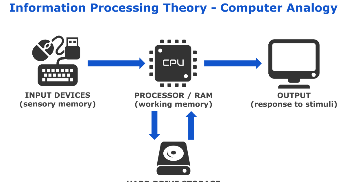
Table of Contents
- Definition and Core Concepts of Processing
- Fundamental Definition and Role in Diverse Systems
- Comparison of Processing in Digital and Physical Systems
- Historical Evolution of Processing Techniques
- Disciplinary Variations in Processing Stages
- Types of Processing in Technology
- Primary Categories of Processing in Technology
- CPU Processing Pipelines and Their Stages
- Parallel Processing vs. Sequential Processing: Comparative Analysis
- Processing in Manufacturing and Industry
- Subtractive vs. Additive Manufacturing Processes
- Role of Automation in Processing Industries
- Batch Processing vs. Continuous Processing in Industrial Settings
- Sustainable Processing Methods in Manufacturing
- Data Processing: Methods and Workflows
- ETL (Extract, Transform, Load) Process and Tools
- Machine Learning Data Processing Workflow
- Real-Time Processing vs. Batch Processing
- Processing in Natural and Biological Systems
- Biological Processing Mechanisms and Artificial Equivalents
- Ecosystem-Level Nutrient and Energy Processing
- Human Cognitive Processing and Computational Models
Processing serves as the invisible force driving progress in technology, industry, and nature, transforming raw inputs into structured outputs that shape modern civilization. From the silicon circuits of a microprocessor to the metabolic pathways of a cell, its principles underpin every system where matter, energy, or information undergoes systematic alteration. This exploration dissects processing’s fundamental mechanisms—spanning digital computation, manufacturing automation, and biological metabolism—to reveal how its evolution has redefined efficiency, precision, and sustainability across disciplines.
The concept transcends rigid boundaries, adapting to the demands of data-centric algorithms, high-volume production lines, and even the self-regulating cycles of ecosystems. By examining its theoretical foundations, technological implementations, and natural parallels, we uncover a unifying framework that bridges abstract theory with tangible applications. Whether optimizing a CPU pipeline or designing a closed-loop recycling system, processing emerges as both a scientific principle and an engineering imperative.
Definition and Core Concepts of Processing
Processing refers to the systematic transformation of inputs into outputs through structured operations, applicable across natural, physical, and computational domains. In computing, processing involves executing instructions to manipulate data, while in manufacturing, it encompasses techniques to alter materials into usable forms. Natural systems, such as biological metabolism or geological erosion, also rely on inherent processing mechanisms to sustain functionality. The concept unifies diverse fields by emphasizing the conversion of raw inputs into refined outputs through defined procedures, whether algorithmic, mechanical, or biochemical.The efficiency, scalability, and precision of processing vary significantly depending on the system’s nature—digital, physical, or hybrid—each governed by distinct principles and constraints. Understanding these distinctions clarifies how processing is tailored to specific applications, from real-time data analysis in software to high-temperature forging in metallurgy.
Fundamental Definition and Role in Diverse Systems
Processing is the controlled manipulation of inputs to achieve a predetermined outcome, characterized by three core elements:1. Input Acquisition: Gathering raw data, materials, or energy (e.g., sensor readings, unprocessed ore, or chemical reactants).
2. Transformation Logic: Applying rules, algorithms, or physical laws to modify inputs (e.g., computational logic in CPUs, heat application in glassblowing).
3. Output Generation: Producing a refined result (e.g., processed files, fabricated components, or metabolic byproducts).
In computing, processing is synonymous with data manipulation, where inputs (e.g., user commands, sensor data) are transformed via software/hardware into outputs (e.g., rendered graphics, control signals). In manufacturing, processing involves material conversion, such as machining metals or fermenting foods, where physical properties are altered through energy application. Natural systems exhibit processing through biochemical pathways (e.g., photosynthesis converting sunlight into glucose) or geological processes (e.g., erosion reshaping landscapes).
Processing efficiency is defined by the ratio of output quality to input consumption (time, energy, resources), with optimal systems minimizing waste while maximizing precision.
Comparison of Processing in Digital and Physical Systems
The following table contrasts processing in digital systems (discrete, algorithmic) and physical systems (continuous, energy-driven), highlighting their defining characteristics, examples, and outcomes.| System Type | Key Characteristics | Examples | Output |
|---|---|---|---|
| Digital Systems |
|
|
|
| Physical Systems |
|
|
|
The duality of processing—digital vs. physical—reflects a spectrum where hybrid systems (e.g., CNC machines combining digital controls with mechanical cutting) bridge the gap by integrating algorithmic precision with material constraints.
Historical Evolution of Processing Techniques
Processing has evolved from mechanical and analog methods to digital and autonomous systems, driven by advancements in energy utilization, material science, and computational theory. Key milestones include:-
Pre-Industrial Era (Before 18th Century)
- Manual processing dominated, relying on human labor and simple tools (e.g., stone grinding, hand-forging).
- Biological processing (e.g., fermentation for beer/wine) used natural microorganisms.
- Mechanical clocks introduced gear-based processing for timekeeping.
-
Industrial Revolution (1760–1840)
- Introduction of water-powered looms and steam engines, enabling mass production.
- Development of metallurgical processing (e.g., Bessemer process for steel).
- Chemical processing scaled with synthetic dyes and explosives (e.g., Haber-Bosch ammonia synthesis).
-
Electrification and Automation (Late 19th–Mid 20th Century)
- Electric motors replaced steam, increasing processing speed (e.g., assembly lines in Ford’s Model T production).
- Analog computing emerged (e.g., slide rules, differential analyzers) for scientific processing.
- Semiconductor invention (1947) laid groundwork for digital processing.
-
Digital Revolution (1970s–Present)
- Microprocessors (e.g., Intel 4004, 1971) enabled programmable processing in consumer electronics.
- Development of algorithmic processing (e.g., quicksort, 1959; cryptography, RSA 1977).
- Industry 4.0 introduced cyber-physical processing, merging IoT sensors with AI-driven optimization (e.g., predictive maintenance in factories).
- Biological processing advanced with CRISPR gene editing and lab-grown meat (cellular agriculture).
The transition from mechanical processing to digital processing reduced human dependency on physical labor while increasing precision, though physical systems remain critical for material-intensive industries.
Disciplinary Variations in Processing Stages
Processing stages vary by domain, reflecting distinct objectives and constraints. Below are flowcharts for data processing (computing) and food processing (manufacturing), illustrating their procedural differences.### Data Processing Flowchart (Computing)
-
Input Collection
- Sources: Sensors, user input, databases, or APIs.
- Format: Structured (CSV, JSON) or unstructured (text, images).
-
Preprocessing
- Cleaning: Removing noise/duplicates (

Types of Processing in Technology
Processing in technology encompasses diverse methodologies tailored to distinct operational requirements, ranging from real-time data manipulation to complex computational simulations. The categorization of processing types—data processing, signal processing, and computational processing—reflects specialized workflows optimized for efficiency, accuracy, and scalability. Each category leverages unique algorithms, hardware architectures, and optimization techniques to address specific challenges in industries such as telecommunications, artificial intelligence, and scientific research.The evolution of processing paradigms has been driven by advancements in semiconductor technology, parallelization techniques, and emerging computational models. While traditional processing models rely on sequential or pipelined execution, modern systems integrate hybrid approaches to balance latency, throughput, and energy consumption. Understanding these categories and their underlying mechanisms is critical for designing systems that meet the demands of contemporary and future applications.
Primary Categories of Processing in Technology
Processing in technology is broadly classified into three primary categories, each serving distinct functional objectives and operational environments.Data Processing
Data processing involves the collection, manipulation, storage, and dissemination of structured or unstructured information to derive meaningful insights or actions. This category is foundational to databases, business intelligence, and big data analytics, where efficiency in storage retrieval and transformation is paramount. Key operations include filtering, aggregation, normalization, and encryption, often executed through software-defined pipelines or specialized hardware like FPGAs (Field-Programmable Gate Arrays) or ASICs (Application-Specific Integrated Circuits). For example, relational databases employ SQL queries to process tabular data, while NoSQL systems handle semi-structured data like JSON or XML.Signal Processing
Signal processing focuses on the analysis, modification, and synthesis of analog or digital signals to extract or transmit information. This category is critical in telecommunications, audio/video compression, radar systems, and medical imaging. Techniques such as Fourier transforms, wavelet analysis, and digital filtering are applied to convert raw signals into usable data formats. Hardware accelerators like DSPs (Digital Signal Processors) or GPUs (Graphics Processing Units) optimize real-time signal manipulation, while software libraries such as FFTW (Fastest Fourier Transform in the West) or Librosa enable algorithmic processing in digital systems.Computational Processing
Computational processing refers to the execution of mathematical or logical operations to solve complex problems, often involving high-performance computing (HPC) or distributed systems. This category encompasses simulations, machine learning, cryptography, and scientific computing. Workloads may range from matrix multiplications in deep learning to Monte Carlo simulations in physics. Architectures like vector processors, TPUs (Tensor Processing Units), or supercomputers are designed to handle computationally intensive tasks, while frameworks such as CUDA or OpenCL abstract parallel execution across heterogeneous hardware.
CPU Processing Pipelines and Their Stages
Central Processing Units (CPUs) employ pipelining to overlap the execution of multiple instructions, improving throughput while maintaining single-thread performance. A modern CPU pipeline typically consists of five to seven stages, each responsible for a specific task in the instruction lifecycle. Below is a detailed breakdown of the five-stage pipeline, a foundational model in CPU design:
Fetch
The fetch stage retrieves the next instruction from memory using the Program Counter (PC), which holds the address of the current instruction. The PC is then incremented to point to the subsequent instruction. Constraints include pipeline hazards, such as data hazards (when an instruction depends on the result of a previous instruction) and control hazards (e.g., branch mispredictions). Stalls or forwarding mechanisms are employed to mitigate these issues.Decode
In the decode stage, the fetched instruction is translated into control signals and operands that the CPU can execute. This involves interpreting opcode fields, determining register operands, and preparing for the Execute stage. Decoders may also identify immediate values or memory addresses embedded in the instruction. Delays in this stage can arise from complex instruction sets (e.g., x86), necessitating wider or multi-cycle decoders.Execute
The execute stage performs the actual arithmetic or logical operations specified by the instruction. This includes ALU (Arithmetic Logic Unit) operations, shifts, or comparisons. For memory-related instructions, this stage may also compute effective addresses. Data hazards are particularly prevalent here, as subsequent instructions may require results from earlier stages. Techniques like register renaming or out-of-order execution (in superscalar CPUs) help mitigate these delays.Memory Access
This stage handles load/store operations, where data is read from or written to memory. For load operations, data is fetched from the specified address; for store operations, data is written back. The von Neumann bottleneck—the latency between CPU and memory—is a critical constraint, often addressed through caching hierarchies (L1, L2, L3) or prefetching. Cache misses can stall the pipeline, reducing efficiency.Write-Back
Pipelining enhances instruction throughput but introduces structural hazards (e.g., resource conflicts) and control hazards (e.g., branches). Modern CPUs mitigate these through dynamic scheduling, speculative execution, and branch prediction algorithms, achieving CPI (Cycles Per Instruction) values close to 1 in ideal scenarios.
The final stage writes the result of an instruction back to the register file or memory, completing the operation. This ensures that subsequent instructions can access updated values. Write-back stalls may occur if the destination register is also a source operand for a later instruction, requiring register forwarding to resolve dependencies.
Parallel Processing vs. Sequential Processing: Comparative Analysis
The choice between parallel processing and sequential processing depends on the problem’s inherent parallelism, resource constraints, and latency requirements. Below is a structured comparison highlighting their use cases, advantages, limitations, and industry applications.
Criteria Parallel Processing Sequential Processing Use Case Tasks with independent or embarrassingly parallel subproblems, e.g., matrix multiplication, Monte Carlo simulations, or real-time video encoding. Tasks with strict dependencies or low computational complexity, e.g., simple arithmetic, linear searches, or single-threaded scripting. Advantages - Higher throughput via concurrent execution across multiple cores or processors.
- Scalability with increased hardware resources (e.g., GPUs, TPUs, or distributed clusters).
- Reduced latency for I/O-bound tasks through asynchronous operations.
- Simplicity in design and debugging, with deterministic execution flow.
- Lower overhead for small-scale or low-latency applications.
- Better cache locality, reducing memory access bottlenecks.
Limitations - Complexity in synchronization (e.g., race conditions, deadlocks) and load balancing.
- Amdahl’s Law limits speedup for serial portions of the workload.
- Increased power consumption and thermal management challenges.
- Bottlenecks in single-core performance, especially for CPU-bound tasks.
- Inefficiency in resource utilization for multi-threaded applications.
- Limited scalability beyond single-core architectures.
Industry Applications - High-performance computing (HPC) in climate modeling or drug discovery.
- Machine learning (e.g., training neural networks on GPUs/TPUs).
- Real-time systems (e.g., autonomous vehicles, financial trading).
- Scientific simulations (e.g., quantum chemistry, fluid dynamics).
- Embedded systems (e.g., microcontrollers in IoT devices).
- Desktop applications (e.g., word processors, basic compilers).
- Legacy systems or constrained environments (e.g., real-time OS kernels).
- Algorithmic tasks with minimal parallelism (e.g., sorting small datasets).
-
Subtractive Manufacturing (Material Removal Processes)
- Material Inputs: Solid blocks or sheets of metals, plastics, wood, or composites (e.g., aluminum, steel, acrylic).
- Tools & Techniques:
- CNC machining (milling, turning, drilling).
- Waterjet or laser cutting.
- Grinding and polishing for surface finishing.
- End-Product Qualities:
- High precision and surface finish, ideal for complex geometries.
- Material waste generation (up to 90% in some cases).
- Suitable for high-strength, durable components (e.g., aerospace turbine blades, medical implants).
- Limitations:
- Tool wear and energy-intensive operations.
- Design constraints due to material removal constraints.
-
Additive Manufacturing (3D Printing)
- Material Inputs: Powders (metal, plastic, ceramics), liquids (photopolymers), or filaments (thermoplastics).
- Tools & Techniques:
- Selective Laser Melting (SLM) for metals.
- Fused Deposition Modeling (FDM) for plastics.
- Stereolithography (SLA) for resins.
- End-Product Qualities:
- Minimal material waste (near-net-shape production).
- Complex geometries and customization without tooling changes.
- Layer-dependent mechanical properties (anisotropy in some materials).
- Limitations:
- Slower production speeds for large volumes.
- Surface roughness requiring post-processing.
-
Key Comparative Insights
Subtractive methods excel in high-volume, high-precision applications with established materials, while additive manufacturing dominates in prototyping, low-volume production, and highly customized parts. Hybrid approaches (e.g., combining 3D printing with machining) are emerging to leverage both techniques.
-
Automation in Automotive Manufacturing
- Robotics: Welding, painting, and assembly lines (e.g., Tesla’s humanoid robots for battery assembly).
- AI Applications:
- Computer vision for defect detection in car bodies.
- Predictive analytics to minimize downtime in assembly lines.
- Outcomes:
- Reduction in defect rates by up to 70% (source: McKinsey, 2022).
- 24/7 production with reduced labor costs.
-
Automation in Pharmaceutical Processing
- Robotics: Pill encapsulation, sterile packaging, and liquid handling in labs.
- AI Applications:
- Machine learning for drug formulation optimization.
- Automated quality control via spectroscopy and imaging.
- Outcomes:
- Compliance with strict regulatory standards (e.g., FDA’s cGMP guidelines).
- Faster response to supply chain disruptions (e.g., Pfizer’s automated COVID-19 vaccine production).
-
Broader Industrial Benefits
Automation reduces workplace injuries by 85% in high-risk environments (OSHA data) and enables real-time data analytics for process optimization. However, it requires significant initial investment and workforce retraining.
- Higher setup costs per batch.
- Lower operational costs for small-scale production.
- High capital expenditure for infrastructure.
- Lower per-unit costs at scale (economies of scale).
- Pharmaceuticals.
- Textiles.
- Custom manufacturing.
- Petrochemicals.
- Paper and pulp.
- Food and beverage (e.g., soda production).
-
Closed-Loop Systems
Data Processing: Methods and Workflows
Data processing transforms raw data into actionable insights through structured methodologies, enabling organizations to derive meaningful patterns, automate decision-making, and optimize operations. The efficiency of these processes depends on the chosen workflows—whether batch-oriented for large-scale historical analysis or real-time for immediate action—and the tools employed to handle extraction, transformation, normalization, and analysis. Below are key methodologies, their technical implementations, and comparative analyses of processing paradigms.
ETL (Extract, Transform, Load) Process and Tools
The ETL (Extract, Transform, Load) process systematically moves data from source systems into a target repository (e.g., data warehouses or lakes) for analytics. Each stage requires specialized tools and scripting to ensure data integrity, scalability, and performance.Extract Phase
Data is retrieved from disparate sources—databases (PostgreSQL, MySQL), APIs (REST/SOAP), or flat files (CSV, JSON). Tools like Apache NiFi, Python libraries (Pandas, Requests), or SQL queries automate extraction. For example, a Python script using `pandas` fetches CSV data:import pandas as pd
data = pd.read_csv("source_data.csv", encoding='utf-8')Transform Phase
Data undergoes cleaning, enrichment, and structuring. Common techniques include:
- Data cleaning: Handling missing values (`df.fillna(0)`), correcting inconsistencies.
- Aggregation: Grouping records (`df.groupby('category').sum()`).
- Normalization: Scaling features (e.g., Min-Max scaling via `sklearn.preprocessing`).
Load Phase
Processed data is written to destinations like data warehouses (Snowflake, BigQuery) or NoSQL databases (MongoDB). Tools such as Apache Spark (for distributed loading) or SQL `INSERT` statements ensure efficient storage.Pseudocode Example (ETL Pipeline)
BEGIN ETL_PROCESS
EXTRACT:
data = QUERY("SELECT FROM sales_db WHERE date > '2023-01-01'")
OR
data = READ_CSV("transactions.csv")TRANSFORM:
data = CLEAN(data) // Remove duplicates, impute missing values
data = AGGREGATE(data, "region", "SUM(sales)")
data = NORMALIZE(data, "price", MIN_MAX_SCALING)LOAD:
WRITE_TO_WAREHOUSE(data, "analytics_db.sales_summary")
OR
SAVE_AS_PARQUET(data, "processed_data.parquet")
END
Machine Learning Data Processing Workflow
Machine learning pipelines require meticulous data handling to ensure model accuracy and reliability. Below is a structured workflow from raw data ingestion to deployment, including tools and expected outputs at each stage.
Step Purpose Tools/Techniques Output 1. Data Ingestion Collect raw data from sources (databases, logs, IoT devices). Apache Kafka, AWS S3, Python (`pandas`, `requests`), SQL `COPY` commands. Structured/unstructured datasets (CSV, JSON, Parquet). 2. Data Exploration Identify patterns, distributions, and anomalies via statistical analysis. Pandas Profiling, Jupyter Notebooks, SQL `DESCRIBE`, `SUMMARY STATISTICS`. Exploratory Data Analysis (EDA) reports, visualizations (Matplotlib/Seaborn). 3. Data Cleaning Handle missing values, outliers, and inconsistencies to improve model robustness. Scikit-learn (`SimpleImputer`), Pandas (`dropna()`, `interpolate()`), SQL `CASE WHEN`. Cleaned dataset with documented transformations (e.g., "Age imputed with median"). 4. Feature Engineering Create or modify features to enhance predictive power (e.g., binning, encoding). FeatureTools, Pandas (`apply()`, `cut()`), SQL `WINDOW FUNCTIONS`. Feature matrix (X) and target variable (y) ready for modeling. 5. Train-Test Split Partition data into training (70-80%), validation (10-15%), and test (10-15%) sets. Scikit-learn (`train_test_split()`), stratified sampling for imbalanced data. Three distinct datasets with preserved class distributions. 6. Model Training Apply algorithms (e.g., Random Forest, XGBoost) to learn patterns from training data. Scikit-learn, TensorFlow/PyTorch, H2O.ai. Trained model with saved parameters (e.g., `.pkl`, `.h5` files). 7. Hyperparameter Tuning Optimize model performance using validation data. GridSearchCV, Bayesian Optimization, Optuna. Hyperparameter grid with best-performing configuration. 8. Evaluation Assess model accuracy, precision, recall, and generalization. Confusion matrices, ROC-AUC, RMSE (for regression), SHAP values. Performance metrics report and error analysis. 9. Deployment Integrate the model into production systems for real-time or batch predictions. Flask/FastAPI (REST APIs), Docker containers, AWS SageMaker, MLflow. Deployed endpoint with latency benchmarks (e.g., <50ms response time). 10. Monitoring Track model drift, data quality, and performance degradation over time. Evidently AI, Prometheus, custom logging (e.g., `logging` module). Alerts for anomalies (e.g., prediction accuracy drop >10%). Real-Time Processing vs. Batch Processing
Data processing systems differ in their approach to handling data based on latency requirements, scalability, and use cases. Below is a comparative analysis of real-time processing (event-driven) and batch processing (scheduled), highlighting their technical trade-offs.Key Differences
Real-time processing prioritizes low latency (milliseconds to seconds) and event-driven triggers, while batch processing optimizes for cost-efficiency and large-scale historical analysis with higher latency (hours to days).
-
Latency:
- Real-time: Sub-second responses (e.g., fraud detection, stock trading).
- Batch: Minutes to hours (e.g., monthly financial reports, log aggregation).
-
Scalability:
- Real-time: Requires distributed architectures (e.g., Apache Kafka, Flink) to handle high throughput.
- Batch: Scales horizontally via frameworks like Hadoop MapReduce or Spark, but with batch job scheduling overhead.
-
Use Cases:
- Real-time:
- Fraud detection in transactions (e.g., Stripe’s real-time monitoring).
- IoT sensor data analysis (e.g., predictive maintenance in manufacturing).
- Personalized recommendations (e.g., Netflix’s dynamic content suggestions).
Processing in Manufacturing and Industry
Manufacturing and industrial processing represent the backbone of modern production systems, where raw materials are transformed into finished goods through systematic workflows. These processes vary in methodology, efficiency, and environmental impact, with subtractive and additive techniques defining distinct approaches to material manipulation. Automation further revolutionizes these sectors by integrating robotics and artificial intelligence (AI) to optimize operations, reduce human error, and enhance scalability. Meanwhile, sustainable processing methods address growing demands for eco-friendly production, balancing cost-effectiveness with reduced carbon footprints. Below, the distinctions between subtractive and additive manufacturing, the role of automation, and comparative industrial processing models are explored, alongside emerging sustainable techniques.
Subtractive vs. Additive Manufacturing Processes
Subtractive and additive manufacturing employ fundamentally different strategies to shape materials, influencing material selection, tooling requirements, and final product characteristics. Subtractive methods remove excess material to achieve the desired form, while additive techniques build objects layer-by-layer from digital models. Each approach offers unique advantages in precision, waste generation, and applicability across industries.
Role of Automation in Processing Industries
Automation integrates robotics, AI, and machine learning to streamline industrial processing, enhancing efficiency, safety, and quality control. In sectors like automotive and pharmaceuticals, automated systems reduce human intervention in hazardous or repetitive tasks while improving consistency. Robotics handle material handling, assembly, and inspection, whereas AI optimizes predictive maintenance and process parameter adjustments.
Batch Processing vs. Continuous Processing in Industrial Settings
Industrial processing methods are categorized into batch and continuous systems based on production volume, flexibility, and operational costs. Batch processing handles discrete quantities of materials, while continuous processing operates in uninterrupted flows. The choice between the two depends on industry demands, scalability needs, and resource constraints.
Criteria Batch Processing Continuous Processing Production Volume Low to medium (e.g., pharmaceutical batches, custom electronics). High (e.g., petroleum refining, bulk chemicals). Flexibility High adaptability to product variations (e.g., food processing lines). Limited flexibility; optimized for single-product streams. Cost Factors Common Industries Sustainable Processing Methods in Manufacturing
Sustainable manufacturing prioritizes resource efficiency, waste reduction, and energy conservation to mitigate environmental impact while maintaining economic viability. Techniques such as closed-loop systems, renewable energy integration, and lean manufacturing principles are increasingly adopted. These methods yield measurable benefits in carbon emissions, operational costs, and regulatory compliance.
Sustainable processing aligns with the United Nations’ Sustainable Development Goals (SDGs), particularly SDG 9 (Industry, Innovation, and Infrastructure) and SDG 12 (Responsible Consumption and Production). Key strategies include:
- Batch:
- End-of-day financial settlements (e.g., PayPal’s batch processing).
- Customer segmentation for marketing campaigns.
- Data warehousing for business intelligence (e.g., Salesforce Analytics Cloud).
- Complexity
Processing in Natural and Biological Systems
Biological systems exhibit sophisticated processing mechanisms that sustain life, from cellular metabolism to ecosystem-level nutrient cycling. These processes—ranging from enzymatic catalysis to neural signal propagation—share functional parallels with artificial systems but operate under distinct biological constraints. Understanding these mechanisms reveals both the elegance of nature’s designs and their potential to inspire technological innovation. Below, the discussion explores biological processing at molecular, organismal, and ecological scales, emphasizing parallels with artificial systems while highlighting unique biological adaptations.
Biological Processing Mechanisms and Artificial Equivalents
Organisms employ specialized processing pathways to transform inputs into outputs, often with efficiencies unattainable by current artificial systems. Below is a comparative analysis of key biological processes and their artificial counterparts, structured to highlight functional analogies and inherent differences.
Note: While artificial systems often prioritize speed or scalability, biological processes excel in adaptability, energy efficiency, and operation under extreme conditions (e.g., deep-sea enzymes active at 100°C). These trade-offs underscore the complementary nature of bio-inspired engineering.Process Biological Example Artificial Equivalent Key Differences Information Transmission Neural action potentials (electrochemical signals in neurons) Digital/analog signal processing (e.g., transistors in CPUs) - Biological: Parallel, probabilistic, energy-efficient (ATP-dependent), and adaptable via synaptic plasticity.
- Artificial: Serial/parallel (von Neumann architecture), deterministic, and energy-intensive (heat dissipation).
Energy Conversion Photosynthesis (light → chemical energy via chlorophyll) Photovoltaic cells (light → electrical energy via semiconductor junctions) - Biological: Multi-step, low-energy yield (~1–2% efficiency), but self-repairing and scalable via chloroplast replication.
- Artificial: High efficiency (~15–22%), but rigid, non-adaptive, and dependent on rare materials (e.g., silicon).
Material Degradation Enzymatic digestion (e.g., cellulases breaking down cellulose) Chemical catalysis (e.g., acid hydrolysis in industrial biorefineries) - Biological: High specificity, mild conditions (pH, temperature), and reusable enzymes.
- Artificial: Broad-spectrum, often harsh conditions (high temperature/pressure), and non-regenerative catalysts.
Pattern Recognition Immune system (antibody-antigen binding) Machine learning (e.g., convolutional neural networks for image recognition) - Biological: Distributed, adaptive (learns via somatic hypermutation), and energy-efficient.
- Artificial: Centralized, static (requires retraining), and computationally expensive.
Waste Recycling Nitrogen fixation (conversion of atmospheric N₂ to ammonia by bacteria) Habers-Bosch process (industrial ammonia synthesis via iron catalysts) - Biological: Ambient conditions, but slow (kinetically limited); symbiotic relationships enhance efficiency.
- Artificial: High yield (~90%), but energy-intensive (3–5% of global natural gas consumption) and non-renewable feedstocks.
Ecosystem-Level Nutrient and Energy Processing
Ecosystems function as self-sustaining processing units, where energy and nutrients cycle through interconnected pathways. The carbon cycle and nitrogen cycle exemplify how biological, geological, and chemical processes collaborate to maintain equilibrium. Below, the carbon cycle is dissected to illustrate these dynamics, with a focus on key participants and their roles.Ecosystems process carbon through a series of transformations: atmospheric CO₂ is fixed by producers (e.g., plants, algae) via photosynthesis, converted into organic matter, and transferred up the food chain. Decomposers (e.g., fungi, bacteria) break down dead organic material, releasing CO₂ back into the atmosphere or sequestering it in soil as stable compounds (e.g., humus). Human activities, such as deforestation and fossil fuel combustion, disrupt this balance by accelerating carbon release, leading to atmospheric accumulation.
Key participants in the carbon cycle include:
- Producers: Autotrophs that synthesize organic compounds from CO₂ and sunlight.
- Examples: Phytoplankton (marine), trees (terrestrial), and cyanobacteria.
- Consumers: Heterotrophs that obtain energy by consuming organic matter.
- Examples: Herbivores (e.g., deer), carnivores (e.g., wolves), and omnivores (e.g., humans).
- Decomposers: Organisms that break down dead biomass into inorganic nutrients.
- Examples: Fungi (e.g., Agaricus bisporus), bacteria (e.g., Pseudomonas), and detritivores (e.g., earthworms).
- Detritivores: Specialized consumers that feed on detritus (partially decomposed organic matter).
- Examples: Millipedes, crabs, and certain beetles.
- Geological Reservoirs: Long-term carbon stores that regulate atmospheric levels.
- Examples: Sedimentary rock (limestone), permafrost, and ocean sediments.
Nitrogen Processing in Ecosystems
The nitrogen cycle similarly relies on microbial mediation to convert nitrogen between its various forms (N₂, NH₃, NO₃⁻). Critical steps include:
- Nitrogen Fixation: Conversion of atmospheric N₂ to ammonia (NH₃) by diazotrophs (e.g., Rhizobium bacteria in legume roots).
- Nitrification: Oxidation of ammonia to nitrite (NO₂⁻) and nitrate (NO₃⁻) by Nitrosomonas and Nitrobacter.
- Assimilation: Uptake of nitrate by plants to synthesize amino acids and nucleic acids.
- Denitrification: Reduction of nitrate back to N₂ by anaerobic bacteria (e.g., Pseudomonas), completing the cycle.
Disruptions and Human Impact:
- Eutrophication: Excess nitrogen from fertilizers triggers algal blooms, depleting oxygen in aquatic systems.
- Soil Degradation: Over-farming reduces microbial diversity, impairing nitrogen cycling.
- Climate Feedback: Permafrost thaw releases stored organic nitrogen, accelerating greenhouse gas emissions.
Human Cognitive Processing and Computational Models
Human cognition relies on dynamic, distributed processing systems that integrate sensory input, memory, and decision-making. These mechanisms exhibit properties—such as parallelism, plasticity, and energy efficiency—that contrast sharply with traditional computational models. Below, a side-by-side comparison highlights the interplay between biological cognition and artificial neural networks (ANNs), emphasizing both convergences and divergences.Biological Cognitive Processing vs. Computational Models
Cognitive Function Biological Mechanism Artificial Equivalent (ANNs) Key Differences Memory Encoding Hippocampal synaptic plasticity (long-term potentiation/depression) and protein synthesis. Weight matrices in ANNs (e.g., backpropagation for training). Biological: Context-dependent, associative, and energy-efficient (~10⁻¹⁹ J per synapse). Artificial: Static unless retrained; energy-costly (GPU/TPU clusters). Attention Mechanisms Prefrontal cortex and basal ganglia modulate focus via dopamine and acetylcholine. Attention layers (e.g., Transformer models’ multi-head attention). Biological: Adaptive, goal-directed, and influenced by emotional state. Artificial: Rule-based, data-dependent. Decision-Making Ventromedial prefrontal cortex integrates rewards, risks, and social cues. Reinforcement learning (RL) agents (e.g., Q-learning, policy gradients). Biological: Intuitive, heuristic Processing is more than a technical process—it is the linchpin of innovation, where the intersection of computation, material science, and biology continuously pushes the limits of what is achievable. From the deterministic steps of a CPU pipeline to the adaptive resilience of biological enzymes, its adaptability demonstrates how systems, whether artificial or natural, evolve to meet complex challenges. As emerging fields like quantum computing and sustainable manufacturing redefine traditional paradigms, the study of processing offers not just solutions but a roadmap for future-proofing industries and ecosystems alike. Understanding its mechanics is not merely academic; it is essential for harnessing its potential to address global demands with precision and foresight.
- Cleaning: Removing noise/duplicates (
Leave a Comment
Comments are moderated before appearing. The data you submit is processed according to the Privacy Policy of viralcontentbee.com.