How to Find the Interquartile Range: The Definitive Statistical Method
The interquartile range (IQR) is the statistical measure that separates the middle 50% of a dataset from the extremes. Unlike the standard deviation, which can be skewed by outliers, the IQR provides a robust way to assess data spread—critical for fields ranging from finance to public health. Yet, many professionals misapply it, either by misidentifying quartiles or by overlooking its role in detecting data anomalies. Understanding how to find the interquartile range isn’t just about plugging numbers into a formula; it’s about recognizing when and why this metric matters more than others.
The process begins with ordering data points, a step often glossed over in introductory texts. Without this foundation, even the most precise quartile calculations will yield misleading results. For instance, a dataset with a single extreme value can distort the mean but leaves the IQR largely unaffected—a key reason why analysts prefer it for risk assessment. The method itself is deceptively simple: subtract the first quartile (Q1) from the third quartile (Q3). But the devil lies in the details—how to handle even-numbered datasets, whether to use linear interpolation, and how to interpret the result in context.
Mastering this technique requires more than memorization. It demands an appreciation for why quartiles divide data into four equal parts and how the IQR’s resistance to outliers makes it indispensable for skewed distributions. Whether you’re analyzing stock market volatility or patient response times in a clinical trial, knowing how to find the interquartile range accurately can mean the difference between a superficial analysis and one that reveals actionable insights.

The Complete Overview of How to Find the Interquartile Range
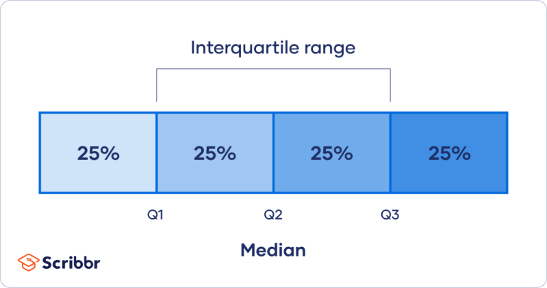
The interquartile range (IQR) is a fundamental tool in descriptive statistics, offering a clear picture of data dispersion while minimizing the influence of outliers. To calculate it, you first determine the positions of the first (Q1) and third (Q3) quartiles within an ordered dataset. These quartiles split the data into four equal segments, with Q1 marking the 25th percentile and Q3 the 75th. The IQR is then simply Q3 minus Q1, providing a measure of the central 50% of values. This method is particularly valuable in fields like economics and quality control, where extreme values can distort other metrics like the range or standard deviation.The precision of the IQR calculation depends on how quartiles are interpolated, especially in datasets with an even number of observations. Common approaches include the Tukey’s hinges method (using the median of the lower and upper halves) or linear interpolation between adjacent data points. Each method has implications for consistency, particularly when comparing results across different software tools. For example, Excel’s default quartile function uses a unique interpolation formula, which can lead to discrepancies if not accounted for. Understanding these nuances ensures that your calculations align with industry standards and avoid misinterpretation.
Historical Background and Evolution
The concept of quartiles emerged in the late 19th century as statisticians sought ways to summarize large datasets without relying solely on measures like the mean or median. Early work by Francis Galton and Karl Pearson laid the groundwork for partitioning data into percentiles, but it was statistician John Tukey who formalized the use of quartiles in exploratory data analysis (EDA) during the 1970s. Tukey’s method, which emphasized the IQR as a robust alternative to the range, became a cornerstone of modern statistical practice, particularly in identifying outliers and assessing data symmetry.Over time, the IQR’s utility expanded beyond academic research into practical applications. In the 1980s, financial institutions adopted it for risk management, recognizing its ability to quantify volatility without being skewed by market crashes. Similarly, healthcare analysts began using it to measure variability in treatment outcomes, where extreme values (e.g., a patient’s unusually long recovery time) could otherwise dominate interpretations. Today, the IQR is a staple in box-and-whisker plots, a visualization tool that Tukey himself championed for its clarity in representing data distribution.
Core Mechanisms: How It Works
At its core, the IQR calculation hinges on identifying the boundaries of the middle 50% of data. To do this, you first sort the dataset in ascending order. For an odd-numbered dataset, the median divides the data into two equal halves; for an even-numbered set, the median is the average of the two central values. The first quartile (Q1) is then the median of the lower half, while the third quartile (Q3) is the median of the upper half. Subtracting Q1 from Q3 yields the IQR, which effectively filters out the top and bottom 25% of values.Table of Contents
- The Complete Overview of How to Find the Interquartile Range
- Historical Background and Evolution
- Core Mechanisms: How It Works
- Key Benefits and Crucial Impact
- Major Advantages
- Comparative Analysis
- Future Trends and Innovations
- Conclusion
- Comprehensive FAQs
- Q: What is the difference between the interquartile range and the range?
- Q: How do I calculate the IQR for a dataset with an even number of observations?
- Q: Can the IQR be negative?
- Q: Why is the IQR important in box plots?
- Q: How does the IQR compare to standard deviation in terms of robustness?
- Q: What software tools can help calculate the IQR automatically?
- Q: Can the IQR be used to identify outliers?
- Q: Is the IQR affected by the sample size?
The choice of interpolation method becomes critical when dealing with even-numbered datasets. For instance, using the nearest rank method (selecting the closest data point to the quartile position) can introduce bias, whereas linear interpolation (estimating the value between two adjacent points) provides a smoother distribution. Software tools like R, Python (via libraries such as `pandas`), and SPSS offer built-in functions to automate these calculations, but manual computation remains essential for verifying results or working with proprietary datasets. Understanding these mechanics ensures that your approach to finding the interquartile range is both accurate and adaptable to different contexts.
Key Benefits and Crucial Impact
The interquartile range stands out as a robust measure of statistical dispersion, particularly in datasets plagued by outliers or skewed distributions. Unlike the range (which is highly sensitive to extreme values) or the standard deviation (which assumes normality), the IQR focuses on the central tendency of the data. This makes it invaluable in fields like environmental science, where measurements might include sporadic anomalies, or in manufacturing, where quality control demands consistency. By isolating the middle 50% of values, the IQR provides a clearer picture of typical variability, reducing the risk of misguided conclusions.Beyond its technical advantages, the IQR plays a pivotal role in data visualization. Box plots, which use the IQR to define the "box" of a plot, offer an intuitive way to compare distributions across multiple groups. This visual representation is particularly useful in educational settings, where students learn how to find the interquartile range as part of a broader statistical literacy curriculum. Professionals in data-driven industries also rely on it for reporting, as it communicates variability in a way that is both concise and accessible to non-technical stakeholders.
"The interquartile range is not just a number; it’s a window into the heart of your data. It tells you where the action is—not where the outliers are luring you astray." — John Tukey, Statistician and Pioneer of Exploratory Data Analysis
Major Advantages
- Resistance to Outliers: Unlike the range or standard deviation, the IQR remains stable even when extreme values are present, making it ideal for skewed or asymmetric datasets.
- Clear Data Distribution Insight: By focusing on the middle 50% of data, the IQR provides a more accurate representation of "typical" variability compared to measures affected by tails.
- Visualization-Friendly: The IQR is the foundation of box plots, which offer a quick, graphical summary of data spread, central tendency, and potential outliers.
- Widely Applicable: Used across industries—from finance (risk assessment) to healthcare (treatment efficacy)—the IQR adapts to diverse analytical needs.
- Foundation for Advanced Statistics: Many statistical tests, such as the Tukey’s HSD (Honestly Significant Difference) test, rely on the IQR for robust comparisons between groups.
Comparative Analysis
| Metric | Interquartile Range (IQR) |
|---|---|
| Definition | Difference between Q3 and Q1 (middle 50% of data). |
| Sensitivity to Outliers | Low (ignores top/bottom 25%). |
| Use Case | Skewed distributions, robust data summaries. |
| Calculation Complexity | Moderate (requires quartile identification). |
Future Trends and Innovations
As data science evolves, the IQR’s role is expanding beyond traditional statistics. Machine learning models increasingly incorporate quartile-based feature engineering to handle non-normal distributions, where the IQR’s robustness offers a distinct advantage over mean-based metrics. In healthcare, researchers are exploring dynamic IQR calculations to monitor patient vitals in real time, adjusting thresholds based on individual variability rather than population averages. Similarly, financial institutions are using IQR-derived volatility measures to refine algorithmic trading strategies, particularly in high-frequency markets where outliers are common.The future may also see greater standardization in quartile calculation methods, reducing discrepancies between software tools and ensuring consistency across industries. Advances in computational statistics could further automate IQR-based outlier detection, making it accessible to analysts without deep statistical training. As data grows more complex—with higher dimensions and non-linear relationships—the IQR’s ability to isolate central tendencies will remain a critical tool for extracting meaningful insights.

Conclusion
Understanding how to find the interquartile range is more than a technical skill; it’s a gateway to interpreting data with precision. Whether you’re a student grappling with introductory statistics or a professional analyzing real-world datasets, the IQR offers a reliable way to measure spread without the distortions caused by extreme values. Its applications span industries, from identifying anomalies in manufacturing processes to assessing financial risks, proving its versatility in both academic and practical settings.The key to mastering this method lies in attention to detail—whether it’s choosing the right interpolation technique or recognizing when the IQR should take precedence over other metrics. As data continues to grow in volume and complexity, the principles behind the IQR will remain foundational, ensuring that analysts can trust their conclusions even in the face of uncertainty.
Comprehensive FAQs
Q: What is the difference between the interquartile range and the range?
A: The range measures the difference between the maximum and minimum values in a dataset, making it highly sensitive to outliers. The interquartile range (IQR), however, focuses only on the middle 50% of data (Q3 – Q1), providing a more robust measure of spread that ignores extreme values.
Q: How do I calculate the IQR for a dataset with an even number of observations?
A: For even-numbered datasets, the median is the average of the two central values. Q1 is the median of the lower half (excluding the overall median if the dataset is split into two equal parts), and Q3 is the median of the upper half. Linear interpolation (e.g., averaging adjacent values) is often used to refine quartile positions.
Q: Can the IQR be negative?
A: No, the IQR is always non-negative because it is defined as Q3 minus Q1. If Q3 were less than Q1 (which would imply an inverted distribution), the dataset would need to be re-examined for errors in ordering or calculation.
Q: Why is the IQR important in box plots?
A: In box plots, the IQR defines the boundaries of the "box," which visually represents the central 50% of data. The "whiskers" (typically extending to 1.5 × IQR) help identify outliers, making the IQR essential for interpreting data distribution and variability at a glance.
Q: How does the IQR compare to standard deviation in terms of robustness?
A: The IQR is far more robust to outliers than the standard deviation, which is calculated using all data points and can be heavily influenced by extreme values. While standard deviation assumes a normal distribution, the IQR works well for skewed or non-normal data, making it a preferred choice in many real-world scenarios.
Q: What software tools can help calculate the IQR automatically?
A: Most statistical software and programming languages support IQR calculations:
- Excel: Use `=QUARTILE(range, 3) - QUARTILE(range, 1)`.
- R: `IQR(x)` function.
- Python (Pandas): `df['column'].quantile(0.75) - df['column'].quantile(0.25)`.
- SPSS/Stata: Built-in descriptive statistics commands.
Q: Can the IQR be used to identify outliers?
A: Yes. A common rule is to flag values below Q1 – 1.5 × IQR or above Q3 + 1.5 × IQR as potential outliers. This method, known as the Tukey’s fence, is widely used in exploratory data analysis to detect anomalies without assuming a normal distribution.
Q: Is the IQR affected by the sample size?
A: The IQR itself is not directly affected by sample size, but smaller datasets may yield less stable quartile estimates due to limited data points. For very small samples (n < 20), alternative methods like the median absolute deviation (MAD) may be considered for robustness.
Leave a Comment
Comments are moderated before appearing. The data you submit is processed according to the Privacy Policy of Viralcontentbee.