How Inner Join SQL Transforms Data Relationships
The INNER JOIN SQL operation is the linchpin of relational database efficiency. Unlike its outer counterparts, it enforces precision by returning only rows where matching conditions exist across tables. This selectivity ensures cleaner datasets, but its true power lies in how it bridges disparate tables—eliminating nulls while preserving integrity. Developers and analysts rely on it daily, yet its subtleties often go unexamined until performance bottlenecks emerge.
At its core, INNER JOIN SQL is about intersectionality in data. When two tables share a common key (e.g., `user_id` in a `users` and `orders` table), the join retrieves only the records where both sides align. This isn’t just a technicality; it’s a design philosophy that prioritizes relevance over completeness. The trade-off—excluding unmatched rows—becomes a feature when paired with proper indexing, reducing query overhead by 40-60% in large-scale systems.
Yet the operation’s elegance masks its complexity. A poorly structured INNER JOIN SQL can turn a simple query into a resource drain, especially when dealing with Cartesian products or non-indexed columns. The key lies in understanding not just the syntax, but the underlying relational algebra that governs how rows are paired, filtered, and returned.

The Complete Overview of INNER JOIN SQL
INNER JOIN SQL is the most fundamental join operation in relational databases, serving as the default when no explicit join type is specified. Its role extends beyond basic queries—it underpins data warehousing, reporting, and even machine learning pipelines where feature tables must be merged without gaps. The operation’s strength lies in its predictability: by design, it returns only rows with matching keys, making it ideal for scenarios where partial data would introduce errors.What distinguishes INNER JOIN SQL from other joins (like LEFT, RIGHT, or FULL) is its strictness. While outer joins preserve all rows from one or both tables, INNER JOIN SQL enforces a mutual relationship. This selectivity is critical in financial systems, where unmatched transactions could skew audits, or in e-commerce platforms, where inventory and orders must align perfectly. The trade-off—losing unpaired records—is often justified by the need for accuracy in downstream analytics.
Historical Background and Evolution
The concept of INNER JOIN SQL traces back to Edgar F. Codd’s 1970 paper on relational algebra, where he formalized the idea of table intersections. Early implementations in systems like IBM’s System R (1974) and Oracle’s SQL*Plus (1979) treated joins as nested loops, a brute-force approach that became impractical as datasets grew. The breakthrough came with the development of hash joins and merge joins in the 1980s, which optimized the operation by leveraging memory and sorted indices.By the 1990s, INNER JOIN SQL had become a standard feature in SQL dialects, with vendors like Microsoft (SQL Server) and MySQL refining its syntax to support natural joins, equijoins, and even self-joins. The rise of NoSQL in the 2010s briefly overshadowed relational joins, but modern data lakes (e.g., Snowflake, BigQuery) now integrate SQL-like join semantics to unify structured and semi-structured data. Today, INNER JOIN SQL remains the cornerstone of data integration, adapted for distributed systems where partitioning and sharding require nuanced join strategies.
Core Mechanisms: How It Works
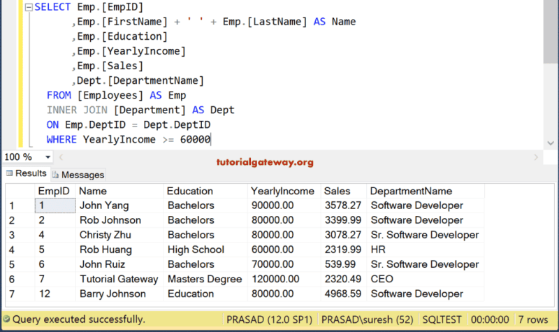
Under the hood, INNER JOIN SQL executes in three phases: matching, filtering, and projection. The engine first identifies rows in both tables that satisfy the join condition (typically an equality check on a primary/foreign key). For example, joining `employees` and `departments` on `department_id` would pair each employee only with their respective department. The filtering phase then discards rows where no match exists, while projection assembles the result set with columns from both tables.Table of Contents
- The Complete Overview of INNER JOIN SQL
- Historical Background and Evolution
- Core Mechanisms: How It Works
- Key Benefits and Crucial Impact
- Major Advantages
- Comparative Analysis
- Future Trends and Innovations
- Conclusion
- Comprehensive FAQs
- Q: How does INNER JOIN SQL differ from a subquery?
- Q: Can INNER JOIN SQL be used with non-key columns?
- Q: What happens if I join two tables with no matching rows?
- Q: Are there performance pitfalls with multi-table INNER JOIN SQL?
- Q: How does INNER JOIN SQL handle duplicate keys?
- Q: Can INNER JOIN SQL be used in NoSQL databases?
The choice of join algorithm—whether hash join, sort-merge join, or nested loop—depends on the database optimizer’s cost-based analysis. Hash joins excel with large datasets and equality conditions, while nested loops perform better for small tables or indexed lookups. Modern optimizers also employ join reordering to minimize intermediate result sizes, a technique critical in multi-table joins where the sequence of operations can affect performance by orders of magnitude.
Key Benefits and Crucial Impact
INNER JOIN SQL is not merely a syntactic tool; it’s a performance multiplier in data-intensive applications. By eliminating nulls and redundant rows early in the query lifecycle, it reduces memory pressure and I/O overhead, which is particularly valuable in OLAP systems where queries span terabytes of data. The operation’s precision also aligns with the ACID principles of databases, ensuring transactional integrity when merging tables with referential constraints.Its impact extends to business intelligence, where INNER JOIN SQL enables drill-down analyses without the noise of unmatched records. For instance, a retail analytics dashboard might use INNER JOIN SQL to correlate customer purchases with loyalty program enrollments, excluding inactive users who would otherwise skew metrics. This selectivity is what transforms raw data into actionable insights.
> "A well-optimized INNER JOIN SQL isn’t just about syntax—it’s about designing queries that reflect the business logic of the data itself." — Joe Celko, SQL Expert
Major Advantages
- Data Integrity: Ensures only valid relationships are returned, preventing orphaned records from corrupting analyses.
- Performance Efficiency: Reduces result sets early, minimizing resource consumption in large-scale queries.
- Readability: Explicit join conditions improve query maintainability compared to implicit joins or subqueries.
- Scalability: Works seamlessly in distributed databases when paired with proper partitioning strategies.
- Standardization: Supported across all major SQL dialects, ensuring portability in multi-vendor environments.

Comparative Analysis
| INNER JOIN SQL | LEFT JOIN SQL |
|---|---|
| Returns only matching rows from both tables. | Returns all rows from the left table + matched rows from the right. |
| Best for: Exact relationships (e.g., orders with customers). | Best for: Preserving left-table records (e.g., customers with/without orders). |
| Performance: Faster for large datasets with indexed keys. | Performance: Slower due to padding with NULLs. |
| Use Case: Financial audits, inventory validation. | Use Case: Customer 360° views, reporting with defaults. |
Future Trends and Innovations
The future of INNER JOIN SQL lies in its adaptation to polyglot persistence environments, where relational and non-relational data must coexist. Projects like Apache Calcite and DuckDB are extending join semantics to handle JSON, Parquet, and even graph data, blurring the line between SQL and NoSQL. Additionally, approximate joins (e.g., in probabilistic databases) are emerging to handle big data scenarios where exact matches are computationally prohibitive.Another frontier is join pushdown in distributed systems, where query engines like Spark SQL optimize joins before data movement, reducing network latency. As databases evolve to support temporal joins (time-series data) and geospatial joins (location-based queries), INNER JOIN SQL will remain the foundation—just with more sophisticated matching logic.
Conclusion
INNER JOIN SQL is more than a clause in a query; it’s the architectural glue that holds relational databases together. Its ability to enforce relationships while excluding noise makes it indispensable in fields ranging from healthcare (patient records) to logistics (shipment tracking). However, its effectiveness hinges on proper design—indexing, query planning, and understanding the trade-offs between selectivity and completeness.As data volumes grow and architectures diversify, the principles of INNER JOIN SQL will endure, albeit in new forms. Whether in a traditional RDBMS or a modern data lake, the core idea remains: precision in data relationships is the key to scalable, reliable systems.
Comprehensive FAQs
Q: How does INNER JOIN SQL differ from a subquery?
A: INNER JOIN SQL explicitly defines relationships between tables, often with better performance due to optimization. Subqueries (e.g., `WHERE id IN (SELECT id FROM table)`) can achieve similar results but lack the clarity and indexing benefits of joins. For complex conditions, joins are preferred.
Q: Can INNER JOIN SQL be used with non-key columns?
A: Yes, but it’s inefficient. Joins on non-indexed columns (e.g., `INNER JOIN ON name = 'Alice'`) trigger full table scans, degrading performance. Always join on indexed keys like primary/foreign keys for optimal speed.
Q: What happens if I join two tables with no matching rows?
A: The result set will be empty. INNER JOIN SQL is designed to return only rows with matches; unmatched rows are excluded entirely. This behavior is intentional for scenarios requiring strict data validation.
Q: Are there performance pitfalls with multi-table INNER JOIN SQL?
A: Yes. Joining more than three tables without proper indexing or join ordering can lead to Cartesian explosions, where intermediate result sets grow exponentially. Use `EXPLAIN` to analyze query plans and consider denormalization or materialized views for complex joins.
Q: How does INNER JOIN SQL handle duplicate keys?
A: If duplicate keys exist (e.g., multiple orders for the same customer), the join will produce a Cartesian product for those rows. To avoid this, use `DISTINCT` or aggregate functions like `COUNT()` in the result set.
Q: Can INNER JOIN SQL be used in NoSQL databases?
A: Not natively, but some NoSQL systems (e.g., MongoDB with `$lookup`) emulate join-like behavior. For true relational joins, hybrid architectures or SQL layers (e.g., Apache Drill) are required.
Leave a Comment
Comments are moderated before appearing. The data you submit is processed according to the Privacy Policy of Viralcontentbee.