How a Box Plot Example Reveals Hidden Data Patterns
The first time a box plot example appears in a dataset, it doesn’t just present numbers—it tells a story. Unlike bar charts that stack categories or line graphs that trace trends, a box plot example compresses an entire distribution into a compact visual framework. It reveals where data clusters, where it stretches, and where it abruptly cuts off—often exposing anomalies that traditional summaries like mean or median would obscure. This is why data scientists and analysts rely on it: a single box plot example can communicate more about variability, skewness, and outliers than pages of raw statistics.
Yet for many, the box plot remains an enigma—a geometric shape that seems to defy intuitive interpretation. The rectangle, the line inside it, the whiskers extending outward—each element carries precise meaning. Misinterpret a box plot example, and you might misdiagnose a dataset’s health. Get it right, and you unlock insights into performance gaps, quality control thresholds, or even market segmentation strategies. The challenge lies in decoding its language without falling into common pitfalls, such as conflating the median with the mean or ignoring the role of the interquartile range (IQR) in defining "normal" behavior.
What follows is an examination of how box plot examples function as both a diagnostic tool and a narrative device. From their origins in exploratory data analysis to their modern applications in machine learning and business intelligence, this guide dissects their mechanics, advantages, and limitations. Along the way, we’ll explore why a well-constructed box plot example can be more persuasive than a spreadsheet—and how to avoid the pitfalls that turn clarity into confusion.

The Complete Overview of Box Plot Examples
A box plot example is more than a statistical chart; it’s a snapshot of data’s personality. At its core, it distills five key metrics into a single visual: the median, the quartiles (Q1 and Q3), the interquartile range (IQR), and the potential outliers. The "box" itself represents the middle 50% of the data (Q1 to Q3), while the "whiskers" extend to 1.5 times the IQR beyond these quartiles. Any data points beyond the whiskers are flagged as outliers, often plotted individually. This structure allows analysts to assess symmetry, skewness, and the presence of extreme values at a glance—a capability no summary statistic can match.The power of a box plot example lies in its ability to compare distributions across categories or time periods. For instance, a marketer analyzing customer spending might use a box plot example to compare purchase behavior across regions, instantly spotting which markets have higher variability or skewed distributions. Similarly, a quality control engineer could deploy box plot examples to monitor production consistency, identifying batches where defects cluster. The versatility stems from its adaptability: it can represent a single dataset or juxtapose multiple groups, making it indispensable in fields from healthcare to finance.
Historical Background and Evolution
The box plot’s origins trace back to John Tukey, the pioneering statistician who popularized exploratory data analysis (EDA) in the 1960s and 1970s. Tukey’s work emphasized visualizing data distributions to uncover patterns before applying formal tests. His "box-and-whisker plot" was designed to complement other tools like stem-and-leaf plots, offering a quick way to grasp central tendency and dispersion. Initially, box plot examples were manual, drawn by hand on graph paper, but their adoption grew as computing power improved, transforming them into a staple of statistical software like R and Python.Over time, the box plot example evolved beyond its exploratory roots. In the 1980s and 1990s, as business intelligence tools emerged, box plots became a standard feature in dashboards, enabling non-statisticians to interpret data trends. Today, they’re embedded in platforms like Tableau and Power BI, often customized with colors or annotations to highlight specific insights. The modern box plot example isn’t just a tool for analysts—it’s a communication device, bridging the gap between raw data and actionable decisions.
Core Mechanisms: How It Works
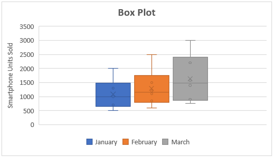
The anatomy of a box plot example is deceptively simple, but each component serves a distinct purpose. The box’s bottom and top edges correspond to the first (Q1) and third quartiles (Q3), respectively, encapsulating the interquartile range (IQR). The line inside the box marks the median (Q2), revealing whether the distribution is symmetric or skewed. Whiskers extend to the smallest and largest values within 1.5 × IQR from Q1 and Q3, while outliers—points beyond this range—are plotted individually. This structure ensures that even a cursory glance at a box plot example can reveal whether data is tightly clustered or widely dispersed.Table of Contents
- The Complete Overview of Box Plot Examples
- Historical Background and Evolution
- Core Mechanisms: How It Works
- Key Benefits and Crucial Impact
- Major Advantages
- Comparative Analysis
- Future Trends and Innovations
- Conclusion
- Comprehensive FAQs
- Q: What’s the difference between a box plot example and a violin plot?
- Q: Can a box plot example show correlations between variables?
- Q: How do I handle extreme outliers in a box plot example?
- Q: Why does my box plot example look asymmetric?
- Q: Are box plot examples useful for time-series data?
The magic happens when comparing multiple box plot examples side by side. For example, in a clinical trial, researchers might use box plot examples to compare treatment efficacy across patient groups, instantly identifying which group shows lower variability in outcomes. The key is interpreting the relative positions: a box plot example with a longer whisker on the right suggests a right-skewed distribution, while overlapping boxes indicate similar central tendencies. The challenge is avoiding misinterpretations—for instance, assuming the median is the "typical" value when outliers skew the data.
Key Benefits and Crucial Impact
Box plot examples excel where other visualizations falter. While histograms show frequency distributions, they struggle with comparing multiple groups. Scatter plots reveal relationships but drown in high-dimensional data. Box plot examples, however, condense complexity into a digestible format, making them ideal for exploratory analysis. Their ability to highlight outliers and skewness in one glance is unmatched, especially in fields like manufacturing, where process control hinges on detecting deviations early.The impact extends beyond technical analysis. In business, a box plot example can justify pricing strategies by revealing customer willingness to pay across segments. In academia, it clarifies research findings by illustrating variability in experimental results. Even in everyday contexts, such as sports analytics, box plot examples help coaches assess player performance consistency. The tool’s versatility stems from its balance of simplicity and depth—a quality that makes it indispensable across disciplines.
"Data visualization is about telling stories with numbers. A box plot example doesn’t just show data; it whispers where the story might twist."
— Edward Tufte, Data Visualization Expert
Major Advantages
- Compact Representation: A box plot example encapsulates an entire distribution in a single frame, making it ideal for comparing multiple datasets without visual clutter.
- Outlier Detection: By flagging points beyond 1.5 × IQR, box plot examples reveal anomalies that could indicate errors, fraud, or rare events.
- Skewness and Symmetry Insights: The relative positions of the median and quartiles expose distribution shape, helping identify skewed or bimodal data.
- Scalability: Works equally well for small datasets (e.g., lab results) or large-scale analyses (e.g., national survey responses).
- Integration with Other Tools: Seamlessly combines with statistical tests (e.g., ANOVA) or machine learning pipelines to validate assumptions.

Comparative Analysis
| Box Plot Example | Alternative Visualization |
|---|---|
| Best for comparing distributions across categories. | Histograms show frequency but lack comparative depth. |
| Highlights outliers and skewness clearly. | Scatter plots reveal relationships but obscure distribution shape. |
| Works with ordinal or continuous data. | Bar charts are limited to categorical comparisons. |
| Scalable for large datasets. | Line graphs struggle with high variability. |
Future Trends and Innovations
As data volumes grow, box plot examples are evolving to handle complexity. Interactive versions now allow users to hover over whiskers to see exact values or filter outliers dynamically. In machine learning, box plot examples are being used to monitor model performance drift, with automated alerts triggered when distributions shift unexpectedly. Future innovations may include AI-driven annotations, where the plot itself suggests hypotheses (e.g., "This skew may indicate a data collection bias").The rise of big data also demands more sophisticated variants. For instance, "notched box plots" provide confidence intervals around the median, while "violin plots" combine box plot examples with kernel density estimates for smoother distributions. These advancements ensure that the tool remains relevant in an era where data isn’t just big—it’s multidimensional.
Conclusion
A well-crafted box plot example is more than a chart; it’s a lens through which data reveals its true character. By distilling complex distributions into a few geometric elements, it empowers analysts to ask the right questions—whether about product quality, market trends, or scientific phenomena. The key to mastery lies in understanding its mechanics: the median’s position, the IQR’s width, and the outliers’ location all tell a story if you know how to listen.Yet the tool’s value extends beyond technical proficiency. In an age where data drives decisions, the ability to interpret a box plot example becomes a critical skill—one that separates insight from intuition. As the examples here demonstrate, its power isn’t just in the numbers but in the narratives they unlock.
Comprehensive FAQs
Q: What’s the difference between a box plot example and a violin plot?
A box plot example focuses on quartiles and outliers, while a violin plot overlays a kernel density estimate to show the full distribution shape. Violin plots are better for visualizing probability densities, whereas box plot examples excel at comparative analysis.
Q: Can a box plot example show correlations between variables?
No. A box plot example is univariate or used for group comparisons but cannot depict relationships between two variables. For correlations, use scatter plots or correlation matrices.
Q: How do I handle extreme outliers in a box plot example?
Outliers beyond 1.5 × IQR are typically plotted individually. For extreme cases, consider using a modified box plot (e.g., Tukey’s "fences") or transforming the data (e.g., log scaling) before visualization.
Q: Why does my box plot example look asymmetric?
Asymmetry (skewness) occurs when the median isn’t centered between Q1 and Q3. Right-skewed data has a longer right whisker; left-skewed data has a longer left whisker. This indicates a distribution tail in one direction.
Q: Are box plot examples useful for time-series data?
Box plot examples can summarize time-series distributions (e.g., monthly sales variability), but they don’t show trends over time. For temporal patterns, combine them with line charts or moving averages.
Leave a Comment
Comments are moderated before appearing. The data you submit is processed according to the Privacy Policy of Viralcontentbee.