Understanding cumulative binomial probability essentials

Table of Contents
- Cumulative Binomial Probability: Mathematical Foundations and Applications
- Mathematical Formulation of Cumulative Binomial Probability
- Comparison of Single-Point and Cumulative Binomial Probabilities
- Step-by-Step Calculation of P(X ≤ 3) for n = 10 and p = 0.4
- Distinction Between Binomial, Uniform, and Normal Distributions
- Applications of Cumulative Binomial Probability in Real-World Scenarios
- Quality Assurance and Acceptance Sampling
- Sports Analytics and Performance Prediction
- Clinical Trials and Binary Outcome Assessment
- Computational Methods and Tools for Cumulative Binomial Probability
- Comparison of Computational Methods for Cumulative Binomial Probability
- Python Implementation for Cumulative Binomial Probability
- binom.cdf(k-1, n, p) computes the cumulative probability up to k-1 successes
- Excel Implementation for Cumulative Binomial Probability
- Generating PMF and CDF Plots in R
- FAQ
- cumulative binomial probability table?
- cumulative binomial probability formula?
- cumulative binomial probability calculator?
- cumulative binomial probability table pdf?
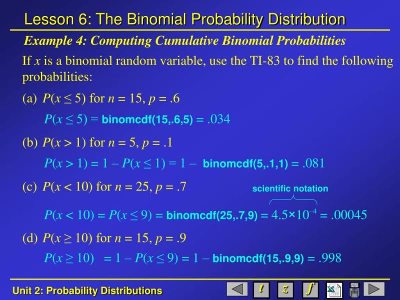
- cumulative binomial probability ti 84?
- cumulative binomial probability function?
The cumulative binomial probability serves as a fundamental tool in statistical analysis by quantifying the likelihood of observing a specified number of successes within a fixed series of independent trials. Unlike single-point probabilities, this approach aggregates outcomes to address real-world questions such as "what is the chance of at least three successes in ten attempts?" or "how likely is it to exceed two failures in a sample of fifty?" By leveraging the probability mass function and cumulative distribution function, practitioners can model discrete events with precision, bridging theoretical frameworks and practical decision-making.
At its core, cumulative binomial probability relies on three key parameters: the number of trials, the probability of success per trial, and the threshold for cumulative evaluation. Whether assessing quality control thresholds, predicting sports outcomes, or evaluating clinical trial efficacy, this method provides a structured way to interpret binary data. Its versatility extends across industries, offering insights where discrete events dominate—from manufacturing defect rates to medical treatment success metrics. The distinction between cumulative and single-point probabilities further refines analytical rigor, ensuring accurate risk assessments and strategic planning.
Cumulative Binomial Probability: Mathematical Foundations and Applications
The cumulative binomial probability represents a fundamental concept in discrete probability theory, enabling the calculation of probabilities for compound events in binomial experiments. Unlike single-point probabilities, which assess the likelihood of a specific number of successes, cumulative binomial probability evaluates the probability of observing up to or at least a certain number of successes in n independent trials. This distinction is critical in fields such as quality control, risk assessment, and experimental design, where decision-making relies on aggregated outcomes rather than isolated events.The binomial distribution models scenarios with fixed trials (n), two possible outcomes (success/failure), and a constant probability of success (p). While the probability mass function (PMF) quantifies the likelihood of exactly k successes, the cumulative distribution function (CDF) extends this to cumulative probabilities, such as P(X ≤ k) or P(X ≥ k). Below, the mathematical framework and practical distinctions between these approaches are explored.
Mathematical Formulation of Cumulative Binomial Probability
The cumulative binomial probability is derived from the binomial PMF, which describes the probability of k successes in n trials:> Binomial PMF:
> \[
> P(X = k) = \binom{n}{k} p^k (1-p)^{n-k}, \quad k = 0, 1, 2, \dots, n
> \]
> where:
> - \(\binom{n}{k}\) is the binomial coefficient (number of combinations),
> - p is the probability of success on a single trial,
> - \(1-p\) is the probability of failure.
The cumulative binomial CDF for P(X ≤ k) is computed by summing the PMF from k = 0 to k = k:
> Cumulative Binomial CDF (Lower Tail):
> \[
> P(X \leq k) = \sum_{i=0}^{k} \binom{n}{i} p^i (1-p)^{n-i}
> \]
For the upper tail (P(X ≥ k)), the complement rule is applied:
\[
P(X \geq k) = 1 - P(X \leq k-1)
\]
Key parameters:
Comparison of Single-Point and Cumulative Binomial Probabilities
The following table contrasts single-point binomial probabilities (PMF) with cumulative probabilities (CDF), highlighting their mathematical expressions, parameter roles, and practical applications.| Parameter | Single-Point PMF: P(X = k) | Cumulative CDF: P(X ≤ k) or P(X ≥ k) | Use Case Example |
|---|---|---|---|
| n (trials) | Fixed number of independent trials (e.g., 10 coin flips). | Same as PMF; defines the range of possible outcomes. | Quality control: Inspecting 50 units for defects (n = 50). |
| k (successes) | Exact count of successes (e.g., k = 3 heads). | Threshold for cumulative evaluation (e.g., P(X ≤ 3) or P(X ≥ 5)). | Reliability testing: Probability of ≤2 failures in 20 trials. |
| p (probability) | Probability of success per trial (e.g., p = 0.3). | Identical to PMF; influences cumulative likelihood. | Marketing: Probability of ≥4 out of 10 customers purchasing a product (p = 0.2). |
| Probability Type | Isolated event probability (discrete point). | Aggregated probability over a range of events. | PMF: "Exactly 3 successes." CDF: "At most 3 successes." |
| Calculation Method | Direct evaluation of \(\binom{n}{k} p^k (1-p)^{n-k}\). | Summation of PMF terms or complement rule for upper tails. | PMF: \(P(X=2)\) in 5 trials. CDF: \(P(X \leq 2)\) or \(P(X \geq 4)\). |
Step-by-Step Calculation of P(X ≤ 3) for n = 10 and p = 0.4
To compute the cumulative probability of observing up to 3 successes in 10 trials with a success probability of 0.4, follow these steps:1. Define the CDF:
\[
P(X \leq 3) = P(X=0) + P(X=1) + P(X=2) + P(X=3)
\]
Each term is calculated using the binomial PMF.
2. Compute Individual PMF Terms:
P(X=0) = \binom{10}{0} (0.4)^0 (0.6)^{10} = 1 \times 1 \times 0.0060466 \approx 0.0060
\]
P(X=1) = \binom{10}{1} (0.4)^1 (0.6)^9 = 10 \times 0.4 \times 0.0100777 \approx 0.0403
\]
P(X=2) = \binom{10}{2} (0.4)^2 (0.6)^8 = 45 \times 0.16 \times 0.0167962 \approx 0.1209
\]
P(X=3) = \binom{10}{3} (0.4)^3 (0.6)^7 = 120 \times 0.064 \times 0.0279936 \approx 0.2150
\]
3. Sum the Probabilities:
\[
P(X \leq 3) = 0.0060 + 0.0403 + 0.1209 + 0.2150 = 0.3822
\]
Thus, the probability of observing 3 or fewer successes in 10 trials is approximately 38.22%.
Distinction Between Binomial, Uniform, and Normal Distributions
The cumulative binomial probability differs fundamentally from uniform and normal distributions in terms of event dependency, parameter constraints, and applicability:Binomial Distribution: Dependency: Trials are independent, with outcomes dependent on a fixed p. Parameters: Discrete, bounded by n trials; success probability p is constant. Use Case: Counting discrete successes/failures (e.g., pass/fail tests, defective items). Key Limitation: Requires finite, identical trials; not suitable for continuous data. - Uniform Distribution:
Dependency: All outcomes are equally likely; no inherent relationship between trials. Parameters: Continuous or discrete; defined by a range (e.g., a to b). Use Case: Modeling randomness without bias (e.g., rolling a fair die, random sampling). Key Limitation: Lacks cumulative probability structure for aggregated events. - Normal Distribution:
Dependency: Continuous, symmetric; outcomes influenced by mean (\(\mu\)) and variance (\(\sigma^2\)). Parameters: Defined by \(\mu\) and \(\sigma\); unbounded range. Use Case: Modeling continuous phenomena (e.g., heights, measurement errors). Key Limitation: Not applicable to discrete counts or fixed-trial experiments. Applications of Cumulative Binomial Probability in Real-World Scenarios
Cumulative binomial probability serves as a foundational tool in quantitative decision-making across disciplines where discrete binary outcomes dominate. Its utility lies in assessing the likelihood of achieving a specified number of successes (or failures) within a fixed number of independent trials, enabling risk mitigation, resource optimization, and evidence-based decision-making. From manufacturing quality control to clinical trial design, this probabilistic framework bridges theoretical modeling with actionable insights, particularly when outcomes are binary and trial counts are finite.The versatility of cumulative binomial distributions stems from their ability to quantify uncertainty in scenarios where events are probabilistic yet structured. Below, four critical applications are examined, each demonstrating how the cumulative binomial probability function (P(X ≤ k)) informs strategic choices, operational thresholds, and hypothesis testing.
Quality Assurance and Acceptance Sampling
In manufacturing and supply chain management, cumulative binomial probability underpins acceptance sampling plans, where batches of products are evaluated based on defect rates. The process involves selecting a random sample of size n from a batch and rejecting the entire batch if the number of defective items exceeds a predefined tolerance level k. The cumulative binomial probability then calculates the risk of incorrectly accepting a batch with an unacceptable defect rate, balancing between producer and consumer risks.Key Parameters and Interpretation
Scenario: Quality control in electronics manufacturing (e.g., testing circuit boards for defects). Key Parameters: n = Sample size (e.g., 50 units). k = Maximum allowable defects (e.g., 2). p = Probability of a defect per unit (e.g., 0.05, based on historical data). Probability Interpretation: The cumulative probability P(X ≤ 2) represents the likelihood that no more than 2 defects are found in the sample of 50 units. Conversely, P(X > 2) quantifies the risk of accepting a batch with more than 2 defects, which may exceed the acceptable quality level (AQL).
Decision-Making Impact: Producer Risk (Type II Error): Probability of rejecting a good batch (e.g., P(X > 2 | p = 0.03)). Consumer Risk (Type I Error): Probability of accepting a bad batch (e.g., P(X ≤ 2 | p = 0.07)). Optimization: Adjust n or k to minimize total inspection costs while maintaining safety margins. Mathematical Formulation
For a batch with true defect probability p, the probability of accepting the batch (i.e., observing ≤ k defects) is:P(X ≤ k) = Σ (from i=0 to k) C(n, i) p^i (1-p)^(n-i)Where C(n, i) is the binomial coefficient. In practice, this is computed using statistical tables or software (e.g., Excel’s `BINOM.DIST` function with cumulative = TRUE).Example
A manufacturer tests 50 circuit boards with an AQL of 2% defects (p = 0.02). The cumulative probability P(X ≤ 2) is approximately 0.9998, indicating a 99.98% chance of accepting the batch if it meets the AQL. If the true defect rate rises to p = 0.05, P(X ≤ 2) drops to 0.7358, increasing the risk of acceptance to an unacceptable level.
Sports Analytics and Performance Prediction
In sports, cumulative binomial probability models the likelihood of achieving a specific number of successes (e.g., free-throw makes, penalty kicks, or successful passes) within a fixed number of attempts. This is particularly useful for game outcome prediction, player evaluation, and strategy optimization. For instance, a basketball player with a 75% free-throw success rate (p = 0.75) may be analyzed for their probability of making at least 15 out of 20 attempts (n = 20, k = 15).Key Parameters and Interpretation
Scenario: Predicting free-throw performance in basketball. Key Parameters: n = Number of attempts (e.g., 20). k = Minimum successful attempts (e.g., 15). p = Success probability per attempt (e.g., 0.75). Probability Interpretation: The cumulative probability P(X ≥ 15) is calculated as 1 – P(X ≤ 14), representing the chance the player makes at least 15 successful throws. For n = 20 and p = 0.75, this is approximately 0.9999, indicating near-certainty of exceeding 15 successes.
Decision-Making Impact: Game Strategy: Coaches may rely on such probabilities to decide when to call timeouts or adjust defensive strategies. Player Scouting: Recruiters evaluate consistency by comparing observed success rates to expected binomial distributions. Betting Markets: Oddsmakers use cumulative binomial models to adjust point spreads or over/under lines based on player performance probabilities. Hypothetical Example
A player with p = 0.75 faces 20 free throws. The probability of making exactly 15 is:P(X = 15) = C(20, 15) (0.75)^15 (0.25)^5 ≈ 0.1762The cumulative probability P(X ≤ 14) is 0.0001, meaning the chance of failing to make at least 15 throws is negligible. However, if p drops to 0.70, P(X ≤ 14) rises to 0.1153, significantly altering strategic decisions.Extensions to Team Performance
For team sports, cumulative binomial distributions can model aggregate outcomes (e.g., total goals scored by a soccer team in a match). If a team scores with probability p = 0.40 per shot and takes 10 shots (n = 10), the probability of scoring at least 6 goals (P(X ≥ 6)) is 0.1121, influencing tactical choices like shot selection or defensive positioning.
Clinical Trials and Binary Outcome Assessment
In clinical research, cumulative binomial probability evaluates the success of treatments with binary outcomes (e.g., cured/not cured, responded/non-responded). This is critical for power analysis, sample size determination, and hypothesis testing in randomized controlled trials (RCTs). The binomial distribution models the number of responders in a treatment group, while cumulative probabilities assess the likelihood of observing a predefined number of successes given a hypothesized effect size.Key Parameters and Interpretation
Scenario: Phase II clinical trial for a new antibiotic. Key Parameters: n = Sample size per group (e.g., 100 patients). k = Minimum responders required for efficacy (e.g., 60). p = Probability of response under treatment (e.g., 0.70 vs. 0.50 for placebo). Probability Interpretation: For the treatment group, P(X ≥ 60) calculates the probability of observing at least 60 responders if the true response rate is 70%. This is compared to the placebo group’s P(X ≥ 60 | p = 0.50) to determine statistical significance.
Decision-Making Impact: Power Analysis: Ensures the trial has sufficient statistical power to detect a true effect (e.g., 80% power at α = 0.05). Interim Analysis: Monitors cumulative success rates to decide on early termination or dose adjustment. Regulatory Approval: Demonstrates efficacy by showing the probability of exceeding a predefined success threshold. Mathematical Formulation for Power
The power of a trial is derived from the cumulative binomial probability under the alternative hypothesis (H₁). For a two-tailed test:Power = 1 – β = P(X ≥ k | H₁) + P(X ≤ (n - k) | H₁)Where β is the Type II error rate. For n = 100, k = 60, and p = 0.70, P(X ≥ 60) ≈ 0.9999, indicating near-certain detection of a 70% response rate.Example: Treatment vs. Placebo Comparison
Treatment Group: p = 0.70, n = 100. P(X ≥ 60) ≈ 0.9999 (high confidence in observing ≥60 responders).
Placebo Group: p = 0.50, n = 100. *P(X ≥
Computational Methods and Tools for Cumulative Binomial Probability
Cumulative binomial probability calculations are foundational in statistical analysis, yet their computational efficiency varies significantly across methods. The choice of approach—whether manual, recursive, software-based, or tabular—directly impacts accuracy, scalability, and practical applicability. This section evaluates computational trade-offs, provides implementation examples in Python and Excel, and explores the limitations of approximations when binomial parameters deviate from ideal conditions for normal approximation.
Comparison of Computational Methods for Cumulative Binomial Probability
The efficiency and feasibility of calculating cumulative binomial probabilities depend on the method employed. Below is a comparative analysis of four primary approaches, structured to highlight their advantages, limitations, and optimal use cases.
Key Consideration: Computational complexity grows exponentially with n for manual and recursive methods, while software and precomputed tools leverage optimized algorithms (e.g., logarithmic transformations or dynamic programming).
Method Pros Cons Best Use Case Manual Summation of PMF Terms
- Conceptual clarity for small n (e.g., n ≤ 20).
- No software dependency; useful for pedagogical purposes.
- Exact results for discrete calculations.
- Time-consuming for large n or k (e.g., n = 100, k = 50).
- Prone to human error in summation.
- No scalability for iterative or real-time applications.
Educational demonstrations, small-scale problems, or environments without computational tools. Recursive Formulas
- Reduces computational steps compared to brute-force summation via recursive relations (e.g., Pascal’s identity).
- Memory-efficient for dynamic programming implementations.
- Exponential time complexity (O(2n)) for naive recursion.
- Risk of stack overflow or performance degradation for n > 30.
- Requires careful implementation to avoid redundant calculations.
Custom algorithmic implementations where iterative optimization (e.g., memoization) is applied, or in constrained environments with limited libraries. Statistical Software (Python/R)
- High precision and speed via optimized C/Fortran libraries (e.g., `scipy` uses regularized incomplete beta functions).
- Supports large n (e.g., n = 106) and edge cases (e.g., p ≈ 0 or 1).
- Integration with visualization and statistical testing frameworks.
- Dependency on external libraries.
- Overhead for trivial calculations.
Professional applications, research, or scenarios requiring reproducibility and scalability. Precomputed Tables or Graphs
- Instant lookup for standard values (e.g., n ≤ 20, p = 0.5).
- Useful in settings with no computational tools (e.g., fieldwork).
- Limited to predefined n, p, and k combinations.
- No flexibility for custom parameters.
- Outdated or incomplete tables may introduce errors.
Quick reference in educational settings or legacy systems with fixed parameters. Python Implementation for Cumulative Binomial Probability
Python’s `scipy.stats` module provides efficient and accurate calculations for cumulative binomial probabilities. Below is a code snippet to compute P(X ≥ 5) for n = 12 and p = 0.3, with detailed comments explaining each step.# Import the necessary library from SciPy
from scipy.stats import binom# Define parameters: number of trials (n), success probability (p), and threshold (k)
n = 12 # Number of independent trials
p = 0.3 # Probability of success on a single trial
k = 5 # Minimum number of successes for P(X ≥ k)# Calculate P(X ≥ k) using the complement rule: P(X ≥ k) = 1 - P(X ≤ k-1)
binom.cdf(k-1, n, p) computes the cumulative probability up to k-1 successes
probability = 1 - binom.cdf(k - 1, n, p)# Print the result with 4 decimal places for clarity
print(f"P(X ≥ {k}) for n={n}, p={p}: {probability:.4f}")Key Notes:
The complement rule (P(X ≥ k) = 1 − P(X ≤ k−1)) avoids summing terms from k to n, improving numerical stability. `binom.cdf` internally uses regularized incomplete beta functions for efficiency, especially for large n. For P(X ≤ k), directly use `binom.cdf(k, n, p)` without the complement. Excel Implementation for Cumulative Binomial Probability
Excel’s statistical functions provide a user-friendly interface for binomial calculations. Below is a step-by-step guide to compute P(X ≤ k) and P(X ≥ k), including conditional formatting for visualization.### Step 1: Input Parameters
1. Enter the following in cells:
A1: `n` (e.g., `12`) B1: `p` (e.g., `0.3`) C1: `k` (e.g., `5` for P(X ≤ 5) or `4` for P(X ≥ 5) via complement). ### Step 2: Compute P(X ≤ k) Use the `BINOM.DIST` function with cumulative set to `TRUE`:
=BINOM.DIST(C1, A1, B1, TRUE)
- Example: For P(X ≤ 5), enter `=BINOM.DIST(5, 12, 0.3, TRUE)` in D2.
### Step 3: Compute P(X ≥ k) Use the complement rule:
=1 - BINOM.DIST(C1 - 1, A1, B1, TRUE)
- Example: For P(X ≥ 5), enter `=1 - BINOM.DIST(4, 12, 0.3, TRUE)` in D3.
### Step 4: Conditional Formatting for Visualization
1. Select the range of cells containing probabilities (e.g., D2:D3).
2. Go to Home > Conditional Formatting > Color Scales.
3. Choose a gradient (e.g., green for higher probabilities, red for lower).
4. Adjust thresholds to highlight probabilities above/below a critical value (e.g., 0.5).
Formula Reference:
`BINOM.DIST(k, n, p, TRUE)`: Cumulative probability P(X ≤ k). `BINOM.DIST(k, n, p, FALSE)`: Probability mass function P(X = k). Excel’s `BINOM.DIST` uses an iterative algorithm optimized for speed, but may lose precision for n > 1000. Generating PMF and CDF Plots in R
R’s `ggplot2` and base graphics functions enable visualization of binomial distributions with annotated probability thresholds. Below is a step-by-step guide to plot the PMF and CDF for n = 12 and p = 0.3, with annotations for P(X ≤ 5) and P(X ≥ 5).From theoretical foundations to computational implementations, cumulative binomial probability demonstrates its indispensable role in transforming raw data into actionable intelligence. By mastering its mathematical underpinnings—such as the interplay between the probability mass function and cumulative distribution function—analysts can navigate complex scenarios with confidence. Real-world applications, spanning quality assurance, sports analytics, and clinical research, underscore its adaptability, while computational tools like Python, R, and Excel streamline calculations for efficiency. As approximations and advanced methods like normal distribution conversions emerge, understanding their limitations ensures robust decision-making. Ultimately, cumulative binomial probability remains a cornerstone of discrete probability theory, empowering professionals to quantify uncertainty and drive evidence-based strategies.
FAQ
cumulative binomial probability table?
Q: What is a cumulative binomial probability table and how do I use it to find probabilities?
cumulative binomial probability formula?
Q: What is the formula for calculating cumulative binomial probability?
cumulative binomial probability calculator?
Q: Where can I find a free online cumulative binomial probability calculator?
cumulative binomial probability table pdf?
Q: How do I download a cumulative binomial probability table in PDF format?
cumulative binomial probability ti 84?
Q: How do I calculate cumulative binomial probability on a TI-84 calculator?
cumulative binomial probability function?
Q: What is the cumulative binomial probability function in Python or Excel?
Leave a Comment
Comments are moderated before appearing. The data you submit is processed according to the Privacy Policy of viralcontentbee.com.