binomial calculator probability essentials for precise

Practical Applications and Use Cases for Binomial Calculators

The versatility of binomial calculators lies in their ability to simplify complex probabilistic assessments into interpretable metrics. Industries leverage them to evaluate success rates, defect probabilities, and system reliability, ensuring compliance with standards while minimizing operational risks. Below, key sectors and scenarios demonstrate their critical role, followed by clarifications on common misconceptions and a case study illustrating real-world impact.

Industries and Fields Utilizing Binomial Calculators

• Manufacturing and Quality Control
  Binomial calculators assess defect rates in production lines, enabling manufacturers to set acceptable quality levels (AQL) and adjust sampling plans. For example, automotive manufacturers use them to determine the probability of a batch failing inspection due to welding defects, ensuring compliance with ISO 9001 standards. A calculator might evaluate the chance of 5% or fewer defective parts in a sample of 100, guiding decisions on whether to reject a shipment or proceed with assembly.
• Healthcare and Clinical Trials
  In medical research, binomial distributions model patient response rates to treatments, such as the probability of a drug achieving remission in a trial. Hospitals use these tools to estimate infection rates post-surgery, helping allocate resources for preventive measures. For instance, a calculator could determine the likelihood of a 2% infection rate in 200 patients, informing whether additional sterilization protocols are necessary.
• Finance and Risk Assessment
  Financial institutions apply binomial models to evaluate default probabilities in loans, fraud detection rates, or the success of marketing campaigns. Insurance companies use them to calculate the probability of claims exceeding expected thresholds, adjusting premiums accordingly. A binomial calculator might assess the chance of 15% of insured vehicles filing claims within a year, guiding underwriting policies.
• Sports Analytics and Performance Evaluation
  Coaches and analysts employ binomial calculators to predict game outcomes based on player success rates, such as free-throw percentages in basketball or penalty kick conversions in soccer. Teams use historical data to compute the probability of winning a match given specific conditions, optimizing strategies. For example, a calculator could estimate the likelihood of a team winning if their star player scores 80% of free throws during a critical game segment.
• Information Technology and System Reliability
  IT departments use binomial distributions to forecast hardware failure rates, software bug detection probabilities, or network outage occurrences. Cloud service providers rely on these tools to ensure 99.9% uptime by calculating the expected number of failures in a system with redundant components. A calculator might determine the probability of a server cluster experiencing more than one failure per month, prompting preventive maintenance.
• Supply Chain and Logistics
  Logistics managers leverage binomial models to assess delivery success rates, inventory shrinkage probabilities, or supplier reliability. For instance, a calculator could evaluate the chance of 10% of shipments arriving late due to weather disruptions, helping optimize routing and contingency plans. Retailers use similar tools to predict stockouts based on demand variability.

Risk Assessment and Probability Evaluation

• Defect Probability in Manufacturing
  Factories use binomial distributions to estimate the likelihood of defective units in a production batch. For example, if a factory produces 1,000 widgets with a known defect rate of 3%, a calculator can determine the probability of finding 40 or more defective units in a sample of 500. This data informs whether to halt production or implement corrective measures, reducing waste and rework costs.
• Failure Rates in Engineering Systems
  Engineers apply binomial models to evaluate the reliability of redundant systems, such as aircraft components or power grids. A calculator might assess the probability of a backup generator failing during a blackout, given its historical success rate of 95%. This helps prioritize maintenance or invest in redundant infrastructure to meet safety standards.
• Fraud Detection in Financial Transactions
  Banks use binomial probability to flag suspicious transactions by calculating the likelihood of an unusual pattern occurring by chance. For instance, if a customer’s transaction success rate is 99.5%, a calculator can compute the probability of 5 fraudulent transactions in 1,000 attempts, triggering alerts for further investigation.
• Drug Efficacy in Pharmaceutical Trials
  Clinical researchers rely on binomial distributions to determine whether a new drug’s success rate exceeds a placebo’s. A calculator might compare the probability of recovery in a treatment group (e.g., 60% success) versus a control group (e.g., 40% success), providing statistical evidence for regulatory approval.
• Customer Churn Prediction in Business
  Companies use binomial models to estimate the probability of customers canceling subscriptions based on historical data. For example, if 5% of customers churn monthly, a calculator can predict the likelihood of 50+ cancellations in a customer base of 1,000, prompting targeted retention strategies.

Common Misconceptions About Binomial Probability

• Assumption of Independence is Always Met
  A frequent error is assuming all trials in a binomial experiment are independent when they are not. For example, predicting the probability of multiple machine failures in a factory without accounting for correlated malfunctions (e.g., due to shared power sources) leads to inaccurate risk assessments. A calculator can highlight discrepancies when observed data deviates from independence, prompting further analysis.
• Fixed Probability Across All Trials
  Many believe the success probability (p) remains constant in real-world scenarios, ignoring variability. For instance, a baseball player’s batting average may fluctuate due to fatigue or pitcher changes. A binomial calculator can adjust for changing probabilities by segmenting trials into homogeneous groups, improving accuracy.
• Ignoring Sample Size Limitations
  Small sample sizes can distort binomial probability estimates, as the approximation to a normal distribution (via the Central Limit Theorem) becomes unreliable. A calculator can signal when np or n(1−p) is insufficient (typically <5) and recommend exact methods like the hypergeometric distribution instead.
• Confusing Binomial with Other Distributions
  Binomial is often mistaken for Poisson (for rare events) or geometric (for first success trials). For example, modeling the number of defects per unit (Poisson) instead of the probability of defects in a sample (binomial) can lead to incorrect quality control decisions. A calculator’s structured input (e.g., fixed n and p) prevents such confusion.
• Overestimating Precision with Limited Data
  Users may rely on binomial probabilities calculated from limited trials, assuming high confidence in results. A calculator can display confidence intervals or require minimum sample sizes to ensure reliable estimates, reducing overconfidence in predictions.

Case Study: Binomial Calculator in Pharmaceutical Quality Control

Context:
A mid-sized pharmaceutical company, MedPharm Inc., faced recurring issues with contamination in its tablet production line, leading to batch rejections and delayed shipments. Historically, contamination rates fluctuated between 1% and 3% per batch, but the company lacked a systematic method to predict rejection probabilities based on real-time data. To address this, MedPharm implemented a binomial probability calculator integrated with its quality management system (QMS).

Implementation:
The calculator was configured to model the probability of contamination exceeding the acceptable threshold of 2% in batches of 5,000 tablets. Key parameters included:

Number of trials (n): 5,000 tablets per batch.

Success probability (p): Variable, based on weekly contamination rates from past 12 months (averaging 1.8%).

Threshold for rejection: ≥100 contaminated tablets (2% of batch size).

The tool also incorporated a cumulative distribution function (CDF) to estimate the probability of exceeding the threshold under different contamination scenarios.

Step-by-Step Guide to Using a Binomial Calculator

The binomial distribution models the probability of achieving a fixed number of successes (k) in n independent trials, each with a constant probability of success (p). A binomial calculator automates computations for exact or cumulative probabilities, parameter estimation, and edge-case scenarios. Mastering its usage ensures accurate statistical analysis in quality control, risk assessment, and experimental design.

Inputting Values and Handling Edge Cases

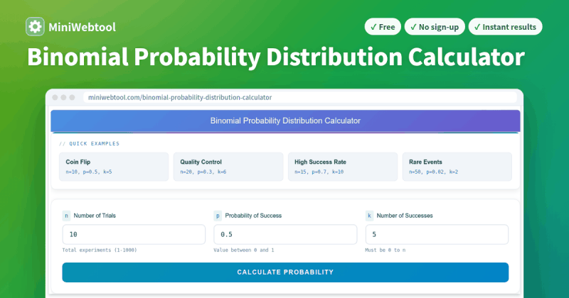
A binomial calculator requires three primary inputs: n (number of trials), k (number of successes), and p (probability of success per trial). Edge cases—such as p = 0.5, k = 0, or k = n—demand special attention due to symmetry or boundary conditions.

To input values:

1. Specify n, k, and p. Ensure n is a positive integer, k is an integer within 0 ≤ k ≤ n, and p is a decimal between 0 and 1.

   Example: For a coin toss (p = 0.5), n = 10 trials, and k = 3 successes, input these values directly.

2. Validate edge cases:
   • p = 0.5: Symmetric distribution; P(X = k) = P(X = n − k). For n = 10 and k = 3, P(X = 3) = P(X = 7).
   • k = 0: Probability of no successes; equivalent to P(X ≤ 0).
   • k = n: Probability of all trials succeeding; equivalent to P(X ≥ n).
   • n = 1: Reduces to a Bernoulli trial; P(X = 1) = p, P(X = 0) = 1 − p.
3. Adjust for cumulative vs. exact probabilities:
   • Exact probability (P(X = k)): Computes the likelihood of exactly k successes.
   • Cumulative probability (P(X ≤ k)): Sums probabilities for 0 to k successes (left-tailed). Use P(X ≥ k) for right-tailed (e.g., 1 − P(X ≤ k − 1)).

   For n = 5, p = 0.3, and k = 2:
   

   Exact: P(X = 2) ≈ 0.3087.

   Cumulative: P(X ≤ 2) ≈ 0.8369.

Interpreting Calculator Outputs

Outputs from a binomial calculator provide either exact or cumulative probabilities, each serving distinct analytical purposes. Misinterpretation can lead to incorrect conclusions, particularly in hypothesis testing or decision-making frameworks.

Key output interpretations:

1. Exact Probability (P(X = k)):
   • Represents the probability of observing exactly k successes in n trials.
   • Useful for binomial tests or evaluating specific outcomes (e.g., "What is the chance of winning exactly 3 out of 5 games?").

   Formula: P(X = k) = C(n, k) × pᵏ × (1 − p)ⁿ⁻ᵏ, where C(n, k) is the combination of n items taken k at a time.

2. Cumulative Probability (P(X ≤ k)):
   • Sum of probabilities for all outcomes ≤ k; critical for determining thresholds (e.g., "What is the probability of failing ≤ 2 times?").
   • Complements include P(X ≥ k) (right-tailed) and P(X < k) (left-tailed excluding k).

   Example: For n = 8, p = 0.4, and k = 5:
   

   P(X ≤ 5) ≈ 0.9678 (high probability of ≤ 5 successes).

   P(X ≥ 5) = 1 − P(X ≤ 4) ≈ 0.3154.

3. Visualizing Results:
   • Graphical representations (e.g., probability mass functions) clarify distributions. Symmetry around np occurs when p = 0.5.
   • For n = 20, p = 0.5, the distribution peaks at k = 10 with P(X = 10) ≈ 0.1762.

Solving for Unknown Variables

Binomial calculators can estimate parameters (n or p) when given a probability, though exact solutions often require numerical methods or iterative approximations. Limitations arise from non-linear relationships and multiple solutions for p.

Procedures for inverse calculations:

1. Solving for p (given n, k, and P(X ≤ k)):
   • Use iterative methods (e.g., Newton-Raphson) or built-in solvers to find p such that P(X ≤ k) = observed probability.
   • Example: If n = 10, k = 4, and P(X ≤ 4) = 0.95, solve for p ≈ 0.7 (approximate).

   Limitation: Multiple p values may satisfy the equation; context (e.g., p < 0.5 or > 0.5) refines solutions.

2. Solving for n (given k, p, and P(X ≤ k)):
   • Requires trial-and-error or optimization algorithms due to the discrete nature of n.
   • Example: For k = 2, p = 0.3, and P(X ≤ 2) = 0.9, n ≈ 7 (verified via calculator).

   Limitation: No closed-form solution; approximations may be necessary for large n.

3. Practical Constraints:
   • Computational complexity increases with large n or extreme p (e.g., p ≈ 0 or 1).
   • Use approximations (e.g., normal distribution for np ≥ 5 and n(1 − p) ≥ 5) when exact methods fail.

Interactive Table Template for Dynamic Calculations

Below is a pseudo-code template for an HTML table that dynamically computes binomial probabilities based on user inputs. This structure can be implemented with JavaScript for real-time updates.

Comparative Analysis: Binomial vs. Other Probability Distributions

Probability distributions serve as the foundation for modeling uncertainty in quantitative analysis, each tailored to distinct scenarios based on data characteristics and underlying assumptions. The binomial distribution is widely used for discrete outcomes in fixed-trial experiments, but its applicability varies alongside other distributions such as Poisson (for rare events) and normal (for continuous, large-scale phenomena). Understanding these distinctions—including when assumptions break down and how calculators adapt—enables practitioners to select appropriate models and interpret results accurately.

The choice between distributions hinges on trial independence, event rarity, and sample size. Binomial calculators, for instance, enforce strict adherence to fixed n and constant p, but real-world data often deviates from these ideal conditions. Hybrid approaches, such as normal approximations for large n, bridge these gaps, while specialized calculators integrate these methods to maintain robustness. Below, a comparative framework outlines key features, limitations, and practical workarounds for each distribution.

Key Features and Applicability of Binomial, Poisson, and Normal Distributions

A structured comparison of these distributions reveals their unique attributes, ideal use cases, and computational distinctions. The table below summarizes core characteristics, including data type (discrete/continuous), assumptions, and examples, while highlighting how calculators implement each model.

Parameter	Input	Result
Number of Trials (n)		10
Successes (k)		3
Probability of Success (p)		0.5

Feature	Binomial Distribution	Poisson Distribution	Normal Distribution
Data Type	Discrete (integer outcomes: 0, 1, 2, ...)	Discrete (counts of rare events: 0, 1, 2, ...)	Continuous (any real value)
Assumptions	Fixed number of trials (n). Independent trials. Constant probability of success (p). Binary outcomes (success/failure).	Events occur independently. Average rate (λ) is constant over time/space. Events are rare (low probability per trial).	Large sample size (n ≥ 30, by Central Limit Theorem). Symmetry around mean (bell curve shape). No strict requirements for trial independence or binary outcomes.
Probability Mass/Density Function	\( P(X = k) = \binom{n}{k} p^k (1-p)^{n-k} \)	\( P(X = k) = \frac{e^{-\lambda} \lambda^k}{k!} \)	\( f(x) = \frac{1}{\sigma \sqrt{2\pi}} e^{-\frac{1}{2}\left(\frac{x-\mu}{\sigma}\right)^2} \)
Mean and Variance	Mean: \( np \); Variance: \( np(1-p) \)	Mean: \( \lambda \); Variance: \( \lambda \)	Mean: \( \mu \); Variance: \( \sigma^2 \)
Calculator Implementation	Direct computation via combinatorial formulas. Iterative or recursive algorithms for large n. Cumulative distribution functions (CDFs) for probabilities.	Approximations for large λ (e.g., normal approximation). Truncated series expansions for computational efficiency. Dynamic adjustment of λ for time-dependent rates.	Standardized to Z-scores for probability queries. Empirical Rule (68-95-99.7) for quick estimates. Integration of cumulative distributions via numerical methods.
Example Use Cases	Quality control: Defective items in a batch of 100 (n=100, p=0.05). Medical trials: Success rate of a drug in 50 patients (n=50, p=0.7).	Call center arrivals: Average 5 calls/hour (λ=5). Traffic accidents: 3 incidents/week in a high-risk zone (λ=3).	Height/weight measurements in populations. Stock price fluctuations over time.

Handling Violations of Binomial Assumptions and Calculator Adaptations

The binomial distribution’s theoretical rigor often clashes with real-world data, where trials may not be independent, probabilities may vary, or sample sizes are indeterminate. Calculators address these violations through statistical adjustments, approximations, and hybrid models to maintain accuracy without sacrificing usability.

Common Violations and Workarounds:
When assumptions are violated, calculators employ the following strategies:

- Dependent Trials:
Binomial calculators assume independence, but correlated data (e.g., clustered failures) requires alternative models like the multinomial distribution or logistic regression. Some calculators include options to adjust for clustering via quasi-binomial models, which estimate variance inflation.

- Variable Probability (p):
If p fluctuates (e.g., learning effects in experiments), the beta-binomial distribution accounts for uncertainty in p by treating it as a random variable. Calculators may integrate Bayesian methods to update p dynamically.

- Large n and Continuity Correction:
For n > 20 and p not near 0 or 1, the normal approximation to the binomial distribution is valid. Calculators apply a continuity correction (e.g., \( P(X \leq 10) \approx P(X \leq 10.5) \)) to improve accuracy when converting discrete probabilities to continuous normal curves.

- Small p and Rare Events:
When p < 0.05, the Poisson approximation to the binomial distribution simplifies calculations, especially for large n. Calculators automatically switch to Poisson if \( np < 5 \) and \( n \) is large, using the formula:

\( \lambda = np \), then \( P(X = k) \approx \frac{e^{-\lambda} \lambda^k}{k!} \).

Calculator-Specific Adaptations:
Advanced binomial calculators incorporate:

Input validation to warn users about potential assumption violations (e.g., p near 0 or 1 with small n).

Hybrid mode toggles between binomial, Poisson, and normal approximations based on user-specified parameters.

Monte Carlo simulations for cases where analytical solutions are infeasible (e.g., complex dependencies).

Hybrid Approaches and Approximations in Probability Calculators

In scenarios where no single distribution perfectly fits the data, calculators leverage hybrid methods to combine strengths of multiple distributions. These approaches enhance flexibility while maintaining computational efficiency.

Normal Approximation to Binomial:
For large n, the binomial distribution converges to a normal distribution with:

Mean: \( \mu = np \)
Variance: \( \sigma^2 = np(1-p) \)
Standardized variable: \( Z = \frac{X - \mu}{\sigma} \)

Calculators implement this via:

Continuity correction for discrete-to-cont

Advanced Features and Customizations in Binomial Calculators

Modern binomial calculators extend beyond basic probability computations by integrating statistical rigor, customization options, and visualization tools. These enhancements address nuanced scenarios in research, quality control, and decision-making, where standard assumptions (e.g., independence, fixed probability) may not hold. Advanced functionalities—such as confidence intervals, hypothesis testing, and adaptive sampling adjustments—enable users to model real-world complexities, while graphical outputs transform abstract probabilities into actionable insights. Customization further refines applicability, allowing adjustments for finite populations, dependent trials, or batch processing, thereby bridging theoretical models with practical implementation.

Key Advanced Functionalities in Binomial Calculators

Binomial calculators now incorporate statistical tools that extend their utility beyond simple probability calculations. These features are particularly valuable in fields requiring rigorous validation, such as clinical trials, manufacturing quality assurance, and risk assessment.

• Confidence Intervals for Proportions
  Modern calculators compute confidence intervals (e.g., 90%, 95%, 99%) around binomial probabilities, providing a range within which the true population proportion is expected to lie. This is critical for hypothesis testing and decision-making under uncertainty.

  For a sample of 100 trials with 30 successes, a 95% confidence interval for the true probability p might span [0.21, 0.39], indicating the estimated success rate could realistically vary within this range.

• Hypothesis Testing Integration
  Built-in z-tests or t-tests for proportions allow users to compare observed success rates against a hypothesized value (e.g., testing if a new drug’s success rate exceeds 50%). Calculators may also support two-proportion tests to compare independent binomial distributions.
• Graphical Probability Visualizations
  Probability mass functions (PMFs) and cumulative distribution functions (CDFs) are rendered as interactive plots, enabling users to:
  • Identify the most likely number of successes (mode of the distribution).
  • Assess the cumulative probability of achieving at least k successes.
  • Compare theoretical distributions against empirical data (e.g., overlaying observed frequencies with predicted probabilities).

  A PMF plot for n=20 trials and p=0.4 reveals that 8 successes are the most probable outcome, while a CDF plot shows the probability of achieving ≥10 successes is approximately 28%.

• Monte Carlo Simulations
  Some calculators simulate repeated binomial experiments to estimate probabilities when analytical solutions are intractable (e.g., for large n or complex dependencies). This is useful in stochastic modeling and risk analysis.
• Bayesian Updating
  Advanced tools incorporate prior distributions to update probability estimates dynamically, aligning with Bayesian inference. This is particularly useful in iterative decision-making processes, such as A/B testing or adaptive clinical trials.

Customization for Non-Standard Binomial Scenarios

Standard binomial calculators assume independent trials with a fixed probability of success. Real-world applications often deviate from these assumptions, requiring adjustments to the underlying model. Customization options address scenarios such as sampling without replacement, dependent trials, or stratified populations.

• Finite Population Correction (Sampling Without Replacement)
  When sampling from a finite population (e.g., inspecting 5% of a batch of 1,000 items), the probability of success changes with each trial. Calculators apply the finite population correction factor:

  Adjusted probability = p × (N−n)/(N−1), where N is the population size and n is the sample size.

  For example, drawing 10 items from a batch of 100 with a defect rate of 10% yields a corrected probability of 0.091 for the first draw and 0.082 for the second.
• Dependent Trials (Markovian or Autocorrelated Successes)
  In scenarios where trial outcomes influence subsequent probabilities (e.g., contagion effects in epidemiology or learning curves in education), calculators may support Markov chain models or autocorrelation adjustments. These require specifying transition probabilities between states (e.g., success → success, success → failure).
• Stratified or Weighted Trials
  Calculators can assign different success probabilities to distinct subgroups (e.g., male vs. female respondents in a survey). This is implemented via weighted binomial distributions, where the overall probability is a function of subgroup proportions and their individual p values.
• Batch Processing and Parameter Sweeps
  Users can automate calculations across multiple parameter sets (e.g., varying n from 10 to 100 while holding p constant) to identify sensitivity thresholds or optimize decision criteria. Outputs may include tables or dynamic plots summarizing results.

Interpretive Value of Visual Outputs in Binomial Calculators

Graphical representations in binomial calculators serve as bridges between raw data and intuitive understanding. They highlight distribution properties, identify outliers, and facilitate comparisons across scenarios. Common visualizations include:

• Probability Mass Function (PMF) Plots
  Bar charts display the likelihood of each possible number of successes (0 to n), revealing skewness, modality, and the most probable outcome. For p close to 0.5, the distribution is symmetric; deviations (e.g., p=0.1) create right-skewed curves.
• Cumulative Distribution Function (CDF) Plots
  Step plots show the probability of achieving k or fewer successes, aiding in threshold analysis (e.g., determining the minimum number of trials needed to exceed a 90% success probability).
• Q-Q Plots for Goodness-of-Fit
  These plots compare observed frequencies against expected binomial probabilities, helping users assess whether real-world data adheres to the binomial model. Deviations may indicate over-dispersion (variance > mean) or under-dispersion.
• Interactive Sliders for Parameter Exploration
  Dynamic interfaces allow users to adjust n and p in real time, observing how changes affect the distribution shape, mean, and variance. This is particularly useful in educational settings or exploratory data analysis.

Hypothetical Ideal Binomial Calculator: Feature Breakdown

An "ideal" binomial calculator would integrate the following advanced capabilities to serve as a versatile tool for statisticians, researchers, and practitioners:

Core Functionalities:

Multi-Distribution Support: Seamless switching between binomial, hypergeometric, and negative binomial distributions, with automatic adjustment for sampling scenarios (e.g., with/without replacement).

Batch Processing: Input of multiple parameter sets (e.g., n×p matrices) for parallel computation, with exportable results in CSV, JSON, or LaTeX formats.

API and Scripting Access: RESTful API or Python/R integration for programmatic use, enabling automation in workflows (e.g., pulling data from databases or IoT sensors).

Real-Time Collaboration: Cloud-based sharing of calculations with annotations, version control, and permission settings for team-based projects.

Statistical Rigor:

Advanced Hypothesis Testing: Support for one-tailed/two-tailed tests, effect size calculations (Cohen’s h), and post-hoc power analysis.

Bayesian Modules: Predefined priors (e.g., Beta distributions) for Bayesian updating, with options to specify custom priors.

Non-Parametric Alternatives: Robust methods (e.g., permutation tests) for scenarios where binomial assumptions are violated.

Visualization and Reporting:

Customizable Dashboards: Drag-and-drop widgets for PMFs, CDFs, and hypothesis test summaries, with themes (dark/light mode) and export to PDF/PPT.

Animation Tools: Dynamic visualizations of distribution changes as parameters vary (e.g., morphing PMFs for p from 0.1 to 0.9).

Integration with BI Tools: Direct compatibility with Tableau, Power BI, or R Shiny for embedding calculations in larger analytical pipelines.

Edge-Case Handling:

Extreme Values: Specialized algorithms for near-zero or near-one probabilities (e.g., using log-transformations to avoid numerical underflow).

Dependent Trials: Graphical interfaces for defining Markov chains or autocorrelation structures, with validation checks for model stability.

High-Dimensional Data: Support for multi-dimensional binomial experiments (e.g., contingency tables with multiple success criteria

Troubleshooting and Common Errors in Binomial Calculations

Binomial probability calculations are foundational in statistics, yet users frequently encounter errors due to misconfigured inputs or misunderstandings of parameter constraints. These errors often stem from invalid values for n (number of trials), k (number of successes), or p (probability of success per trial), leading to calculator warnings or incorrect results. Addressing these issues requires familiarity with the binomial distribution’s mathematical boundaries and practical validation techniques. Below, structured guidance outlines common pitfalls, error resolution, and verification methods to ensure accurate computations.

Common Input Errors and Calculator Warnings

Users frequently input values that violate the binomial distribution’s fundamental constraints, triggering error messages or illogical outputs. Below is a structured table of typical errors, their causes, and corrective actions.

Error/Warning	Cause	Solution	Example
Invalid probability p	p is outside the range [0, 1].	Ensure p is a decimal between 0 and 1 (e.g., 0.5 for 50% probability).	Input: n = 10, k = 3, p = 1.2 → Error: "Probability must be ≤ 1." Correction: p = 0.6 (valid).
k exceeds n	k (desired successes) is greater than n (total trials).	Adjust k to a value ≤ n. The binomial probability for k > n is mathematically 0.	Input: n = 5, k = 7 → Warning: "Successes cannot exceed trials." Correction: k = 3 (valid).
Non-integer n or k	n or k are not whole numbers.	The binomial distribution requires n and k to be integers. Round or adjust inputs if fractional values are necessary (e.g., use Poisson approximation for large n and small p).	Input: n = 12.5, k = 4 → Error: "Trials must be integer." Correction: n = 12 (or use alternative distribution).
Negative n or k	Inputs are negative, which is invalid.	Ensure n and k are non-negative integers. Negative values imply impossible scenarios.	Input: n = -3, k = 2 → Error: "Trials cannot be negative." Correction: n = 3 (valid).
Floating-point precision errors	Extremely large n or p values near 0/1 cause numerical instability.	Use statistical software (e.g., R’s `dbinom` or Python’s `scipy.stats`) for high-precision calculations or apply logarithmic transformations.	Input: n = 1,000,000, p = 0.000001 → Calculator returns "NaN" due to underflow. Solution: Use `log(dbinom(k, n, p))` in R for stability.

Understanding these errors prevents misinterpretation of results. Calculators typically enforce these constraints programmatically, but users must align inputs with the binomial distribution’s definition: n ≥ k ≥ 0, 0 ≤ p ≤ 1, and n ∈ ℕ.

Validation of Binomial Calculator Outputs

To ensure accuracy, binomial calculator results should be cross-verified using manual calculations, statistical software, or alternative methods. Below are systematic approaches to validation.

Manual Verification Using the Binomial Probability Formula
The binomial probability mass function is:

\[ P(X = k) = \binom{n}{k} p^k (1-p)^{n-k} \]

For small n (e.g., n ≤ 20), compute the probability manually and compare it to the calculator’s output. Example:

For n = 4, k = 2, p = 0.5:
\[ \binom{4}{2} (0.5)^2 (0.5)^{2} = 6 \times 0.25 \times 0.25 = 0.375 \]
Calculator output should match 0.375.

Software-Based Validation
Statistical tools provide robust implementations with error handling. Examples include:

R: `dbinom(k, size = n, prob = p)`

dbinom(2, 4, 0.5) # Output: 0.375

- Python (SciPy): `scipy.stats.binom.pmf(k, n, p)`

from scipy.stats import binom
binom.pmf(2, 4, 0.5) # Output: 0.375

- Excel: `BINOM.DIST(k, n, p, FALSE)`

These tools handle edge cases (e.g., p = 0 or 1) and large n more reliably than basic calculators.

Cumulative Probability Checks
For cumulative probabilities (e.g., P(X ≤ k)), ensure the calculator’s output aligns with the cumulative distribution function (CDF):

\[ P(X \leq k) = \sum_{i=0}^{k} \binom{n}{i} p^i (1-p)^{n-i} \]

Example: For n = 5, k = 1, p = 0.3, the CDF should sum probabilities for k = 0 and k = 1:
\[ P(X \leq 1) = \binom{5}{0} (0.3)^0 (0.7)^5 + \binom{5}{1} (0.3)^1 (0.7)^4 \approx 0.1681 + 0.3602 = 0.5283 \]

Edge Cases in Binomial Calculations

Edge cases test the limits of the binomial distribution’s applicability and calculator robustness. These scenarios often reveal mathematical nuances or implementation quirks.

Case 1: n = 0 (No Trials)
When n = 0, the only possible outcome is k = 0 (no successes). The probability is:

\[ P(X = 0) = \binom{0}{0} p^0 (1-p)^0 = 1 \]

Calculators should return 1 for k = 0 and 0 for k > 0. Example:

Input: n = 0, k = 0, p = 0.5 → Output: 1 (correct).

Input: n = 0, k = 1 → Output: 0 (invalid, as no trials exist).

Case 2: p = 0 or p = 1 (Certainty)

If p = 0, the probability of k successes is 1 if k = 0 and 0 otherwise.

\[ P(X = k) = \begin{cases}
1 & \text{if } k = 0, \\
0 & \text{otherwise.}
\end{cases} \]

If p = 1, the probability is 1 if k = n and 0 otherwise.

\[ P(X = k) = \begin{cases}
1 & \text{if } k = n, \\
0 & \text{otherwise.}
\end{cases} \]
Mastering binomial probability through calculators transforms abstract statistical theory into actionable insights, empowering professionals to mitigate risks, optimize processes, and validate hypotheses with confidence. From manufacturing defect analysis to sports analytics, the versatility of these tools lies in their ability to adapt to diverse industries while maintaining rigorous mathematical integrity. As technology evolves, so too do calculator capabilities—incorporating machine learning for predictive modeling or cloud-based collaboration for team-driven projects. The key to harnessing these advancements lies in understanding not just the mechanics of input and output, but the underlying assumptions and limitations that govern each calculation. By doing so, users can navigate edge cases, troubleshoot errors, and ultimately, make data-driven decisions that align with both statistical accuracy and real-world constraints.

FAQ

How do I calculate binomial probability step by step using a binomial probability calculator?

A binomial probability calculator typically requires four inputs: number of trials (n), probability of success (p), number of successes (k), and the type of probability (e.g., "exactly k", "at least k", or "between a and b"). The calculator then computes the result using the formula:

How do I use a binomial probability calculator on a TI-84 calculator?

On a TI-84, use the `binompdf(` function for exact probabilities or `binomcdf(` for cumulative probabilities. For example, to find the probability of exactly 3 successes in 10 trials with p=0.5, enter `binompdf(10, 0.5, 3)`. For "at least 3," use `1 - binomcdf(10, 0.5, 2)`. Access these functions via 2nd → DISTR in the menu.

What is a good statistics helper for calculating binomial probability?

Free online tools like Stat Trek’s Binomial Calculator, WolframAlpha, or Social Science Statistics (socscistatistics.com) provide step-by-step binomial probability calculations. For offline use, software like R (with `dbinom()` or `pbinom()`), Excel (with `BINOM.DIST`), or graphing calculators (e.g., TI-84) are reliable alternatives.

How do I calculate binomial probability between two numbers, like P(5 ≤ X ≤ 10)?

To find the probability of X between two numbers (e.g., 5 and 10), subtract the cumulative probability up to the lower bound from the cumulative probability up to the upper bound. For example, P(5 ≤ X ≤ 10) = P(X ≤ 10) – P(X ≤ 4). Use a calculator’s cumulative function (e.g., `binomcdf(n, p, 10) – binomcdf(n, p, 4)`).

How do I calculate binomial probability using StatCrunch?

In StatCrunch, go to Stats → Probability → Binomial, then enter the number of trials (n), success probability (p), and the value(s) for X. For cumulative probabilities, check the "Cumulative" box. For ranges (e.g., a to b), calculate P(X ≤ b) – P(X ≤ a–1). StatCrunch displays the result along with the formula used.

What is the best online binomial probability calculator?

Popular online binomial calculators include Calculator.net, Omni Calculator’s Binomial Probability Calculator, and Good Calculators. These tools require inputs for n, p, k, and the probability type (exact, cumulative, or range). They provide instant results with optional step-by-step explanations, though accuracy depends on correct input formatting.