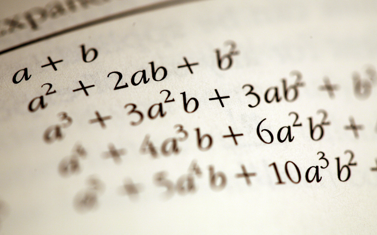
Algebra Story Problem Solver Mastery Through Structured
Published

algebra story problem solver
Table of Contents

Algebraic story problems serve as a bridge between abstract mathematical concepts and real-world applications, demanding both analytical precision and contextual interpretation. An effective algebra story problem solver systematically deciphers narrative challenges, transforming them into structured equations while preserving the integrity of underlying relationships. This process not only enhances problem-solving efficiency but also strengthens conceptual understanding, ensuring learners can apply algebraic principles across diverse scenarios—from financial modeling to scientific simulations.

The functionality of such a solver extends beyond mere computation, incorporating variable identification, equation formulation, and solution validation within a cohesive workflow. By distinguishing between numerical data and contextual cues, these tools eliminate ambiguity, reducing common errors tied to misinterpretation or logical missteps. Whether addressing linear equations, quadratic relationships, or exponential growth, the solver’s adaptability ensures scalability from introductory exercises to advanced real-world case studies.

algebra story problem solver

Definition and Core Functionality of an Algebra Story Problem Solver

An algebra story problem solver is a specialized computational tool designed to bridge the gap between abstract mathematical concepts and real-world scenarios. Its primary purpose is to automate the translation of word-based problems into structured algebraic expressions, enabling users—particularly students, educators, and professionals—to derive solutions efficiently. Unlike rote memorization of formulas, this tool emphasizes contextual understanding, ensuring that numerical data and linguistic cues are accurately interpreted to form solvable equations.

The core functionality revolves around three interconnected processes: variable identification, equation formation, and solution execution. These components work synergistically to decompose a narrative problem into its mathematical essence, leveraging natural language processing (NLP) and symbolic computation. The tool distinguishes between numerical values (e.g., "twice the cost of apples") and contextual relationships (e.g., "total expenditure equals income minus savings") by parsing syntax, semantic roles, and domain-specific keywords. This distinction is critical, as misclassification can lead to incorrect equation formulation—a challenge traditional manual methods often struggle with due to cognitive load.

Key Components of an Algebra Story Problem Solver

The operational workflow of an algebra story problem solver can be segmented into distinct phases, each addressing a specific aspect of problem-solving. These phases are not linear but iterative, with feedback loops to refine interpretations. Below are the foundational components that define its functionality:

1. Natural Language Parsing
The solver begins by analyzing the input text to extract meaningful segments. This involves:

  • Tokenization: Splitting the problem into individual words or phrases (e.g., "John has 3 more apples than Mary" → ["John", "has", "3", "more", "apples", "than", "Mary"]).
  • Part-of-Speech Tagging: Identifying nouns (variables), verbs (operations), and modifiers (quantifiers) to distinguish between entities and actions.
  • Dependency Parsing: Mapping grammatical relationships (e.g., "3" modifies "apples", "more" indicates addition relative to "Mary").
  • 2. Variable and Constant Identification
    The solver maps textual entities to mathematical symbols:

  • Variables: Abstract quantities represented by letters (e.g., "let \( x \) = number of apples John has").
  • Constants: Fixed values (e.g., "3 more apples" → \( x = y + 3 \), where \( y \) is Mary’s apples).
  • Operators: Translating words like "sum", "difference", or "product" into \( +, -, \times \).
  • 3. Equation Formation
    Using parsed components, the solver constructs one or more equations. This step includes:

  • Logical Inference: Combining clauses to form relationships (e.g., "Total cost = price per unit × quantity").
  • Unit Consistency Checks: Ensuring dimensions align (e.g., "miles per hour" vs. "kilometers per second").
  • Constraint Handling: Incorporating inequalities or conditional statements (e.g., "if \( x > 10 \), then discount applies").
  • 4. Solution Execution
    The solver employs algebraic techniques to resolve the equation(s):

  • Symbolic Computation: Applying rules like substitution, elimination, or factoring.
  • Numerical Approximation: For non-linear or transcendental equations, iterative methods (e.g., Newton-Raphson) may be used.
  • Verification: Cross-checking solutions against the original problem to ensure contextual validity.
  • Distinguishing Numerical Data from Contextual Clues

    A critical challenge in solving algebra story problems is differentiating between explicit numerical data and implicit contextual cues. Traditional manual methods rely heavily on human interpretation, which can introduce errors due to ambiguity or misplaced emphasis. Automated solvers address this through systematic analysis:

    Explicit Numerical Data
    These are quantifiable values directly embedded in the problem:

  • Absolute Values: "The train travels 150 miles" → \( \text{distance} = 150 \).
  • Relative Quantities: "Twice as fast as" → \( \text{speed}_\text{train} = 2 \times \text{speed}_\text{car} \).
  • Ratios/Proportions: "3:2 ratio of red to blue marbles" → \( \frac{\text{red}}{\text{blue}} = \frac{3}{2} \).
  • Contextual Clues
    These are linguistic or situational hints that define relationships:

  • Temporal/Sequential: "After 2 hours, the distance covered..." → \( \text{distance} = \text{speed} \times 2 \).
  • Comparative: "Older than", "less than" → Inequalities (\( x > y \)).
  • Domain-Specific Terms: "Profit = Revenue − Cost" (accounting), "Force = Mass × Acceleration" (physics).
  • The solver uses keyword mapping and domain ontologies to classify clues. For example:

  • Temporal keywords ("before", "after", "during") trigger time-based equations.
  • Comparative keywords ("more than", "fewer than") generate inequalities.
  • Domain keywords ("interest rate", "volume") invoke specialized formulas.
  • Example Workflow:
    Problem: "A rectangle’s length is 5 units more than its width. If the perimeter is 30 units, find the dimensions." 1. Parsing: "length = width + 5" → \( L = W + 5 \).
    2. Perimeter Formula: \( P = 2(L + W) = 30 \).
    3. Substitution: \( 2((W + 5) + W) = 30 \) → \( 4W + 10 = 30 \).
    4. Solution: \( W = 5 \), \( L = 10 \).

    Comparison: Manual vs. Automated Solving Methods

    The efficiency and accuracy of algebra story problem solvers can be evaluated against traditional manual methods. Below is a structured comparison highlighting key differences:
    Criteria Traditional Manual Solving Automated Solver
    Input Handling Requires human parsing of text into equations. Prone to misinterpretation of ambiguous phrases. Uses NLP to systematically extract and classify components. Reduces ambiguity through structured analysis.
    Error Identification Errors often go unnoticed until verification (e.g., incorrect variable assignment). Flags inconsistencies (e.g., unit mismatches, logical contradictions) during parsing.
    Scalability Time complexity increases with problem complexity (e.g., multi-step word problems). Handles complex problems efficiently via algorithmic decomposition (e.g., recursive parsing for nested conditions).
    Solution Accuracy Dependent on individual skill; may miss edge cases (e.g., hidden constraints). Consistently applies mathematical rules; reduces human bias in interpretation.
    Learning Aid Encourages critical thinking but may reinforce procedural errors if not guided. Provides step-by-step explanations, highlighting logical transitions between stages.
    Adaptability Limited to familiar problem types; struggles with domain-specific jargon. Customizable with domain ontologies (e.g., physics, economics) to handle specialized terminology.
    Time Efficiency Linear time relative to problem complexity; manual verification adds overhead. Near-constant time for parsing; solution generation scales logarithmically with equation complexity.
    Key Advantage of Automated Solvers:
    The primary efficiency gap lies in redundancy elimination. Manual methods often involve repetitive steps (e.g., re-reading the problem, redefining variables), while automated solvers integrate parsing, equation formation, and solving into a seamless pipeline. Additionally, solvers excel in scalability—handling hundreds of variables or multi-equation systems without degradation in performance, whereas human solvers face cognitive limits.

    Limitations of Automated Solvers:
    Despite advancements, current solvers may struggle with:

  • Highly Ambiguous Problems: Phrases like "more than half" can yield multiple interpretations (\( x > \frac{y}{2} \) vs. \( x \geq \frac{y

    Step-by-Step Problem-Solving Methods for Common Algebraic Story Problems

  • Algebraic story problems transform real-world scenarios into mathematical expressions, requiring systematic translation of language into equations. Mastery of this process involves recognizing patterns in problem structures, assigning variables strategically, and validating solutions through contextual checks. Below are structured methodologies for linear equations, multi-step scenarios, and common pitfalls, ensuring accuracy and efficiency in problem resolution.

    Procedural Guide for Solving Linear Equation Story Problems

    Linear equation story problems typically involve a single unknown and direct relationships between quantities. The following steps ensure a logical progression from problem interpretation to solution validation.

    Step 1: Identify the Unknown
    Begin by pinpointing the primary quantity to solve for. This is often the subject of the question (e.g., "Find the number of apples" or "Determine the total cost"). If multiple unknowns exist, prioritize the one directly asked for or express others in terms of it.

    Step 2: Assign Variables
    Replace the unknown with a variable (e.g., x, y, or descriptive names like A for "apples"). Clearly define the variable in words to avoid ambiguity:

    Let x = the number of students in the class.
    Step 3: Translate Words into Equations
    Convert the problem’s narrative into a mathematical equation using keywords as guides:
  • "More than" → Addition (+)
  • "Less than" → Subtraction (−)
  • "Times as much as" → Multiplication (×)
  • "Divided equally" → Division (÷)
  • "Total" or "Sum" → Addition (= combined value)
  • Example: "A number increased by 5 equals 12" translates to:

    x + 5 = 12
    Step 4: Solve the Equation
    Apply algebraic operations (e.g., inverse operations, distributive property) to isolate the variable. For x + 5 = 12, subtract 5 from both sides:
    x = 12 − 5 x = 7
    Step 5: Validate the Solution
    Substitute the solution back into the original problem context to ensure logical consistency. For the example, verify: "7 increased by 5 equals 12" holds true.

    Techniques for Multi-Step Word Problems

    Multi-step problems (e.g., age-related, mixture, or work-rate scenarios) require breaking down complex relationships into manageable parts. The following strategies streamline variable substitution and equation construction.

    Variable Substitution for Interdependent Quantities
    When two or more unknowns interact (e.g., ages of siblings or concentrations in mixtures), assign variables to each and express relationships between them. For example:

    Let A = Alice’s current age and B = Bob’s current age. Given: Bob is 3 years older than Alice and their ages sum to 31. Equations: 1. B = A + 3 2. A + B = 31
    Substitute the first equation into the second to solve for A:
    A + (A + 3) = 31 2A + 3 = 31 2A = 28 A = 14 B = 17
    Work-Rate Problems
    These involve rates (e.g., "John can paint a room in 5 hours") and combined efforts. Use the formula:
    Work = Rate × Time Total Work = (Rate₁ + Rate₂) × Combined Time
    Example: "Two pipes fill a tank in 3 hours together. Pipe A alone takes 5 hours. Find Pipe B’s time."
    Let t = Pipe B’s time in hours. Pipe A’s rate = 1/5 tank/hour; Pipe B’s rate = 1/t tank/hour. Combined rate: (1/5 + 1/t) = 1/3 (since they fill 1 tank in 3 hours). Solve for t: (t + 5)/(5t) = 1/3 3(t + 5) = 5t 3t + 15 = 5t 15 = 2t t = 7.5 hours
    Mixture Problems
    Focus on the total quantity and proportions of components. Use the formula:
    Total Amount = (Concentration₁ × Volume₁) + (Concentration₂ × Volume₂)
    Example: "How many liters of 30% alcohol solution must be mixed with 50 liters of 70% solution to get a 50% mixture?"
    Let x = liters of 30% solution needed. Total alcohol: 0.3x + 0.7 × 50 = 0.5(x + 50) Solve for x: 0.3x + 35 = 0.5x + 25 10 = 0.2x x = 50 liters

    Validation and Common Pitfalls in Algebraic Story Problems

    Validation ensures solutions align with the problem’s context, while recognizing pitfalls prevents systematic errors. Below are critical checks and corrective actions.

    Validation Through Contextual Substitution
    After solving, replace variables with numerical values in the original problem to confirm logical consistency. For instance, if solving for ages:

    Original statement: "Alice is 14, Bob is 17, and their ages sum to 31." Check: 14 + 17 = 31 (Valid).
    Common Pitfalls and Corrective Actions
    Misinterpretations of language or operational errors often lead to incorrect solutions. The following table outlines frequent mistakes and their resolutions:
    Pitfall Incorrect Translation Correct Approach
    "More than" vs. "Less than" x − 5 for "5 more than x" Use x + 5 for "5 more than x"; x − 5 for "5 less than x".
    Ignoring Units Solving for x without tracking units (e.g., dollars, liters). Include units in variable definitions (e.g., x dollars).
    Overlooking Combined Rates Adding rates directly without considering time (e.g., Rate₁ + Rate₂ instead of Rate₁ × Time + Rate₂ × Time). Use the formula Work = Rate × Time for combined efforts.
    Incorrect Variable Assignment Assigning x to a derived quantity (e.g., x = total cost including tax). Define x as the base quantity (e.g., x = pre-tax cost; 1.08x = total cost).
    Assuming Linear Relationships Treating non-linear scenarios (e.g., area problems) as linear. Identify relationships (e.g., Area = length × width) and adjust equations accordingly.
    Proactive Strategies
  • Diagrams: Sketch visual representations (e.g., number lines for age problems, Venn diagrams for mixtures).
  • Unit Analysis: Track units through each step to ensure dimensional consistency.
  • Peer Review: Verify equations with a colleague to catch translational errors.
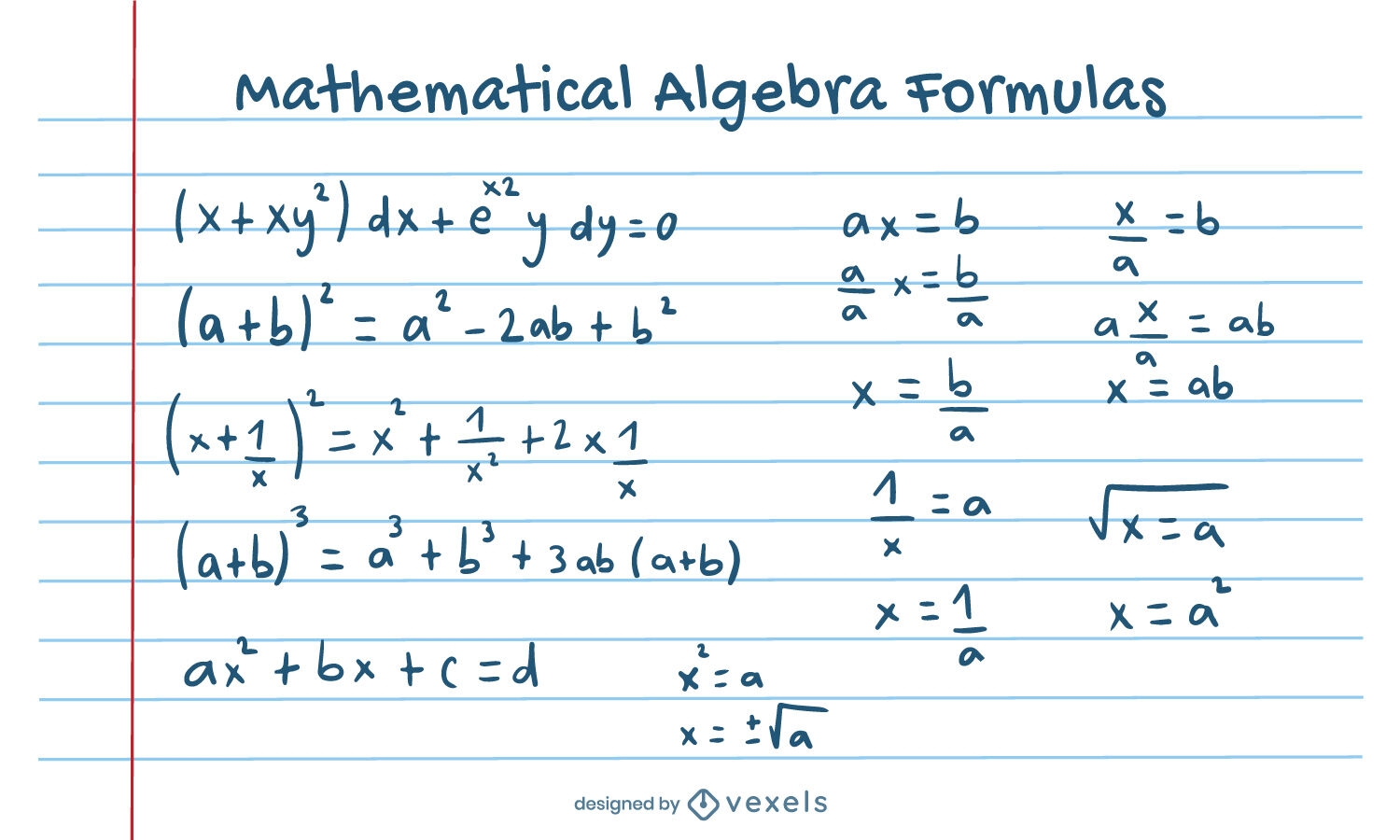
  • algebra story problem solver - Ilustrasi 2

    Advanced Techniques for Solving Complex Algebraic Story Problems

    Algebraic story problems often transcend basic linear relationships, requiring the identification of hidden patterns, nonlinear dependencies, and interconnected systems. Advanced techniques involve translating real-world scenarios into mathematical models—such as quadratic equations, exponential functions, or systems of equations—while ensuring the derived expressions accurately reflect the problem's constraints. These methods are essential for fields like physics, economics, and engineering, where relationships between variables are rarely straightforward. Below, structured approaches address quadratic modeling, exponential growth/decay, and systems of equations, supplemented by real-world case studies demonstrating their practical application.

    Quadratic Modeling in Story Problems

    Quadratic equations arise in scenarios where quantities vary with the square of another variable, such as projectile motion, optimization of areas, or financial profit calculations. The key to solving these problems lies in recognizing the relationship between variables and expressing it in the form ax² + bx + c = 0, where x represents the unknown quantity. Common contexts include:
  • Projectile Motion: Height or distance as a function of time, governed by gravity (e.g., h(t) = -16t² + v₀t + h₀).
  • Area/Perimeter Optimization: Maximizing or minimizing rectangular areas given fixed perimeters (e.g., A = x(10 - x) for a rectangle with perimeter 20).
  • Break-even Analysis: Revenue and cost functions intersecting at a quadratic profit equation.
  • To solve these:
    1. Define Variables: Assign algebraic symbols to unknowns (e.g., time t, side length x).
    2. Formulate the Equation: Translate the scenario into a quadratic expression using known relationships (e.g., Pythagorean theorem for projectile paths).
    3. Solve Using Methods: Apply factoring, completing the square, or the quadratic formula (x = [-b ± √(b² - 4ac)] / 2a).
    4. Validate Solutions: Ensure answers align with physical constraints (e.g., time cannot be negative in motion problems).

    Example: A rectangular garden has a perimeter of 40 meters. If the area is 96 m², find its dimensions.

  • Equation: Let x be the length; width = (40 - 2x)/2 = 20 - x.
  • Area: x(20 - x) = 96 → x² - 20x + 96 = 0.
  • Solution: Factored as (x - 12)(x - 8) = 0, yielding dimensions 12 m × 8 m.
  • Modeling Exponential Growth and Decay

    Exponential functions describe scenarios where quantities change at rates proportional to their current value, such as population growth, radioactive decay, or compound interest. The general form is A(t) = A₀e^(kt) or A(t) = A₀(1 + r)^t, where:
  • A₀ = initial amount,
  • k or r = growth/decay rate,
  • t = time.
  • Key Steps:
    1. Identify the Base Model: Determine if the scenario involves continuous growth (e^(kt)) or discrete intervals ((1 + r)^t).
    2. Extract Parameters: Use given data to solve for A₀, k, or r (e.g., half-life in decay problems).
    3. Formulate the Equation: Incorporate initial conditions (e.g., A(0) = A₀).
    4. Solve for Unknowns: Apply logarithms to isolate variables (e.g., ln(A(t)/A₀) = kt).

    Example: A bacterial culture grows from 500 cells to 2,000 in 3 hours. Find the growth rate k.

  • Equation: 2000 = 500e^(3k) → 4 = e^(3k) → ln(4) = 3k → k ≈ 0.462/hour.
  • General Model: A(t) = 500e^(0.462t).
  • Real-World Application:

  • Finance: Compound interest calculations (A = P(1 + r/n)^(nt)) for investments.
  • Epidemiology: Modeling disease spread (S(t) = S₀e^(-rt) for susceptible populations).
  • Systems of Equations in Story Contexts

    Systems of equations arise when multiple relationships exist between variables, such as shared costs, combined work rates, or supply-demand equilibria. Solving these without guesswork involves:
    1. Variable Definition: Assign distinct symbols to each unknown (e.g., x = cost of item A, y = cost of item B).
    2. Equation Formation: Translate word clues into linear equations (e.g., "three of A and two of B cost $20" → 3x + 2y = 20).
    3. Solution Methods:
  • Substitution: Solve one equation for a variable and substitute into another.
  • Elimination: Add/subtract equations to cancel variables.
  • Matrix Methods: Use Gaussian elimination for larger systems (e.g., AX = B).
  • 4. Verification: Plug solutions back into original equations to ensure consistency.

    Example: A store sells pens for $2 and notebooks for $3. A customer buys 5 items for $13. How many of each?

  • Equations:
  • x + y = 5 (total items),
  • 2x + 3y = 13 (total cost).
  • Solution: Substitute y = 5 - x into the second equation → 2x + 3(5 - x) = 13 → x = 2, y = 3.
  • Advanced Strategy:
    For nonlinear systems (e.g., quadratic + linear), use substitution to reduce complexity. For example:

  • x² + y = 10 and x + y = 6 → Solve the linear equation for y and substitute into the quadratic.
  • Real-World Case Studies: Bridging Theory and Application

    Case 1: Physics – Projectile Trajectory Optimization
    A soccer player kicks a ball at 20 m/s at an angle θ. The height h(t) = -4.9t² + (20 sinθ)t models its trajectory. To maximize range, θ = 45° (derived from range = (v₀² sin(2θ))/g). Algebraic solvers verify optimal angles and predict landing distances, critical for sports analytics and engineering design.
    Case 2: Business – Break-Even Analysis
    A company produces widgets with fixed costs of $5,000 and variable costs of $10 per unit. Revenue is $25 per unit. The break-even point occurs when Total Cost = Total Revenue:
  • 5000 + 10x = 25x → x = 250 units.
  • Algebraic models extend to profit maximization by incorporating quadratic demand functions (e.g., P = 30 - 0.1x).
    Case 3: Environmental Science – Pollution Decay
    A lake’s pollutant concentration decays exponentially: C(t) = C₀e^(-0.1t), where C₀ = 100 ppm. To reduce levels to 50 ppm:
  • 50 = 100e^(-0.1t) → t = ln(2)/0.1 ≈ 6.93 hours.
  • Such models inform cleanup strategies by predicting decay rates under varying conditions.
    Table: Comparative Techniques for Complex Problems
    Problem TypeMathematical ModelKey TechniqueExample Application
    Quadratic Optimizationax² + bx + c = 0Vertex formula (x = -b/2a)Maximizing profit with cost constraints
    Exponential GrowthA(t) = A₀e^(kt)Logarithmic transformationPopulation projections
    Systems of EquationsLinear/Nonlinear pairsSubstitution or matrix methodsSupply-demand equilibrium
    Projectile Motionh(t) = -½gt² + v₀t + h₀Quadratic solvingBallistics trajectory analysis

    Interactive Learning Tools and Visual Aids for Algebraic Story Problem Solving

    Algebraic story problems often require translating real-world scenarios into mathematical expressions, a process that benefits significantly from interactive tools and visual aids. These resources enhance comprehension by providing dynamic representations of abstract concepts, reducing cognitive load, and offering immediate feedback. Digital tools such as graphing calculators, step-by-step solvers, and simulation platforms bridge the gap between theoretical understanding and practical application, while visual aids—such as flowcharts and decision trees—systematically break down complex logical structures. Below, the integration of these tools is explored, alongside their respective strengths, limitations, and pedagogical applications.

    Digital Tools for Visualizing Algebraic Story Problems

    Digital tools transform algebraic story problems into interactive experiences, allowing students to visualize relationships between variables and outcomes. These tools often incorporate real-time graphing, symbolic manipulation, and adaptive feedback, making them particularly effective for problems involving rates, proportions, or systems of equations.

    Key Digital Tools and Their Applications
    Algebraic story problems frequently involve scenarios where variables interact dynamically. Tools such as Desmos Graphing Calculator, GeoGebra, and Wolfram Alpha enable users to input equations derived from story problems and observe their graphical representations instantly. For example:

  • Desmos supports sliders for adjusting parameters (e.g., initial velocity in a projectile motion problem), allowing students to see how changes affect the trajectory.
  • GeoGebra combines algebraic and geometric visualizations, useful for problems involving area, volume, or coordinate geometry.
  • Wolfram Alpha provides step-by-step solutions with explanatory text, ideal for verifying manual calculations.
  • Limitations of Digital Tools
    While powerful, these tools have constraints:

  • Over-reliance on automation may hinder conceptual understanding if students treat them as black-box solvers.
  • Accessibility issues arise for students without internet or compatible devices, exacerbating equity gaps.
  • Static representations (e.g., pre-generated graphs) fail to capture the dynamic nature of some problems, such as those involving iterative processes or conditional logic.
  • Prompt-Based Descriptions for Step-by-Step Solutions
    To illustrate solutions without visuals, descriptive prompts can be structured as follows:
    > *"A student’s notebook shows the following steps for solving a problem about two trains traveling toward each other:
    > 1. Define variables: Let \( t \) = time in hours until collision, \( v_1 \) = speed of Train A (50 mph), and \( v_2 \) = speed of Train B (70 mph).
    > 2. Set up the equation: The combined distance covered by both trains equals 300 miles (their initial separation). Thus, \( 50t + 70t = 300 \).
    > 3. Solve for \( t \): Combine like terms to get \( 120t = 300 \), then divide by 120 to find \( t = 2.5 \) hours.
    > 4. Interpret the result: The trains collide after 2.5 hours, with Train A having traveled \( 50 \times 2.5 = 125 \) miles and Train B \( 70 \times 2.5 = 175 \) miles.
    > The student verifies the solution by checking if \( 125 + 175 = 300 \)."*

    Flowcharts and Decision Trees for Structuring Complex Problems

    Complex algebraic story problems often involve conditional statements, multiple scenarios, or nested dependencies. Flowcharts and decision trees provide structured frameworks to map out logical branches, ensuring clarity in problem-solving pathways. These aids are particularly useful for:
  • Multi-step problems with alternative solutions (e.g., "If the train is delayed, adjust the arrival time by \( x \) hours").
  • Optimization tasks where variables interact under constraints (e.g., maximizing profit given cost and demand functions).
  • Real-world applications such as loan amortization or budget allocation, where conditions (e.g., interest rates) alter outcomes.
  • Designing Effective Flowcharts for Algebraic Problems
    A well-constructed flowchart for an algebraic story problem should:
    1. Start with a clear objective (e.g., "Find the break-even point for a product").
    2. Include decision nodes for conditional logic (e.g., "If revenue > costs, proceed to profit calculation").
    3. Use mathematical annotations within boxes to denote equations or operations (e.g., "Set \( R = 20x \) and \( C = 10x + 500 \)").
    4. End with a solution or conclusion (e.g., "Break-even occurs at \( x = 25 \) units").

    Example: Decision Tree for a Mixture Problem
    Consider a problem where two solutions with different concentrations are mixed to achieve a target concentration. A decision tree might branch as follows:

  • Root: "Determine volumes of Solution A (10% acid) and Solution B (30% acid) to make 100 mL of 20% acid."
  • Branch 1: "Let \( x \) = volume of A, \( y \) = volume of B. Constraint: \( x + y = 100 \)."
  • Branch 2: "Set up equation for acid content: \( 0.10x + 0.30y = 0.20 \times 100 \)."
  • Leaf Node: "Solve the system: \( y = 100 - x \), substitute into acid equation to find \( x = 66.\overline{6} \) mL and \( y = 33.\overline{3} \) mL."
  • Advantages Over Text-Only Approaches
    Flowcharts and decision trees excel in:

  • Reducing cognitive overload by breaking problems into manageable steps.
  • Highlighting dependencies between variables and conditions.
  • Facilitating group work, as visual structures are easier to discuss collaboratively.
  • Comparison of Text-Based and Visual Approaches to Solving Story Problems

    The choice between text-based and visual methods depends on the problem’s complexity, the learner’s strengths, and the available resources. Below is a comparative table outlining their respective strengths and limitations:
    Aspect Text-Based Approach Visual (Diagram/Graph) Approach
    Best For Problems with linear relationships, clear variable definitions, or minimal conditions (e.g., "A car travels 60 mph for 2 hours—find distance"). Problems involving multiple variables, non-linear relationships, or conditional logic (e.g., "A business adjusts prices based on demand—find the optimal price").
    Strengths
    • Encourages abstract reasoning and symbolic manipulation.
    • Portable and requires no additional tools.
    • Develops algebraic fluency through practice.
    • Reveals patterns and relationships intuitively (e.g., intercepts in a graph).
    • Accommodates different learning styles (visual/spatial learners).
    • Supports immediate verification of solutions (e.g., plotting a point to check if it satisfies an equation).
    Limitations
    • Struggles with problems requiring spatial or multi-dimensional reasoning.
    • Can overwhelm learners with complex conditions or nested logic.
    • Lacks dynamic feedback for iterative problem-solving.
    • May obscure algebraic steps if over-relied upon (e.g., "black-box" graphing).
    • Requires proficiency in interpreting visual data (e.g., reading slopes or axes).
    • Creation of diagrams can be time-consuming for hand-drawn solutions.
    Pedagogical Role Foundational for building algebraic intuition and procedural skills. Complements text-based methods by providing concrete representations of abstract concepts.
    Real-World Example
    Solving for the time it takes for two workers to complete a task together:
    *"Worker A completes a job in 5 hours; Worker

    Error Analysis and Debugging in Algebraic Story Problem Solutions

    Algebraic story problems serve as a bridge between real-world contexts and mathematical abstraction, yet common pitfalls—such as unit mismatches, variable misassignments, or misinterpreted keywords—can derail solutions. Systematic error analysis ensures accuracy by identifying recurring mistakes, validating logical consistency, and refining problem-solving strategies. This section explores structured debugging techniques, reverse-engineering flawed solutions, and peer-review checklists to enhance precision in algebraic reasoning.

    Common Pitfalls in Story Problem Solving

    Algebraic story problems often introduce errors due to ambiguities in language or misaligned mathematical interpretations. Below are recurring mistakes categorized by their root causes, along with corrective strategies.
    • Unit Inconsistencies
      Problems involving mixed units (e.g., miles vs. kilometers, dollars vs. cents) frequently lead to incorrect calculations. For example, converting 50 miles to kilometers without proper scaling (1 mile ≈ 1.609 km) results in distorted answers.
      Corrective Template:
      1. Identify all units in the problem and list their conversions (e.g., 1 hour = 60 minutes).
      2. Standardize units to a single system (e.g., metric or imperial) before substitution.
      3. Verify dimensional homogeneity in equations (e.g., ensure both sides of an equation have compatible units).
    • Misassigned Variables
      Assigning variables to incorrect quantities (e.g., letting x represent the total cost instead of the unit price) disrupts the problem’s structure. This often occurs when keywords like "each," "total," or "per" are misinterpreted.
      Example of Misassignment:

      Problem: "A book costs $15 each, and a pack of pens costs $5 total. What is the combined cost for 3 books and 2 packs of pens?"

      Incorrect: Let x = total cost of books and pens (lumps quantities together).

      Correct: Let x = cost per book, y = cost per pack of pens (aligns with "each" and "total").

    • Keyword Misinterpretation
      Words like "more than," "less than," or "combined" can alter the mathematical operation. For instance, "5 more than x" translates to x + 5, not 5x or x − 5.
      Common Keyword Pitfalls:
      KeywordCorrect InterpretationIncorrect Interpretation
      "Total"Sum of quantities (e.g., a + b)Multiplicative factor (e.g., a × b)
      "Each"Per-unit value (e.g., price per item)Aggregate value (e.g., total price)
      "Difference"Subtraction (a − b)Absolute value or ratio (|a/b|)

    Cross-Checking Solutions for Consistency

    Verifying solutions involves rephrasing the problem mathematically and ensuring the derived equation aligns with the original context. This method catches discrepancies such as extraneous solutions or logical contradictions.
    • Rephrasing the Problem Mathematically
      Translate the story problem into an equation using the assigned variables. For example:

      Problem: "A train travels 300 km in 2 hours. How long would it take to travel 450 km at the same speed?"

      Mathematical Rephrase: Speed (s) = Distance (d) / Time (t) → s = 300 km / 2 h = 150 km/h.
      New time (t₂) = 450 km / 150 km/h = 3 hours.

      Compare the rephrased equation with the original problem to confirm logical consistency.

    • Unit and Dimensional Analysis
      Ensure all terms in the equation have compatible units. For instance, in the train example, distance (km) must divide by time (h) to yield speed (km/h). Inconsistent units (e.g., mixing km and miles) invalidate the solution.
    • Plausibility Check
      Assess whether the solution makes sense in the real-world context. For example:

      Problem: "A rectangle’s length is twice its width. Its perimeter is 30 meters. Find the dimensions."

      Solution: Width = 5 m, Length = 10 m (perimeter = 2*(5 + 10) = 30 m).

      Plausibility: Positive dimensions and correct perimeter confirm validity.

    Reverse-Engineering Flawed Solutions

    When a solution fails, systematically dissecting the steps reveals where the logic broke down. This involves tracing back from the final answer to the initial setup, identifying the first incorrect assumption or operation.
    • Step-by-Step Backtracking
      Start from the final answer and work backward to the problem statement. For example:

      Incorrect Solution: For the problem "John has 3 times as many apples as Mary. Together they have 24 apples. How many does John have?", the answer was 18.

      Backtracking:

      1. Final answer: John has 18 apples.
      2. If John has 18, Mary has 24 − 18 = 6 (but 18 ≠ 3 × 6).
      3. Error: Misassigned variables (let x = Mary’s apples, John’s = 3x; equation x + 3x = 24 → x = 6, John = 18).
    • Keyword and Operation Audit
      Review each keyword for correct mathematical translation. For instance:

      Problem: "The sum of two numbers is 10. The difference is 2. Find the numbers."

      Incorrect Setup: x + y = 10 and x − y = 2 (correct), but solving yields x = 6, y = 4.

      Error Detection: If the solver mistakenly wrote x × y = 10, the solution would be invalid. Audit reveals the operation mismatch.

    • Graphical or Tabular Verification
      For problems involving relationships (e.g., rates, proportions), plot the solution on a graph or table to visualize consistency. For example:

      Problem: "A car’s speed increases by 10 km/h every hour. After 3 hours, it reaches 80 km/h. What was its initial speed?"

      Solution: Initial speed = 50 km/h (50 + 10*3 = 80).

      Verification: Create a table showing speed at each hour (50, 60, 70, 80) to confirm linear progression.

    Peer Review Checklist for Story Problem Solutions

    A structured checklist ensures solutions are mathematically accurate, logically coherent, and clearly communicated. Below is a bullet-point guide for peer review, categorized by key evaluation criteria.
    • Problem Interpretation
      • Are all variables clearly defined with units (if applicable)?
      • Do the assigned variables align with the problem’s keywords (e.g., "each," "total")?
      • Is the mathematical setup (equation/inequality) consistent with the problem statement?
    • <

      Adaptive Learning and Personalized Problem Generation in Algebraic Story Problem Solving

      Adaptive learning systems in algebra education dynamically adjust problem complexity, feedback mechanisms, and contextual relevance to align with a learner’s evolving proficiency. These systems leverage algorithms to generate personalized story problems that incrementally challenge the user while reinforcing foundational concepts. By integrating cultural and contextual variations, adaptive platforms ensure broader applicability without compromising the underlying algebraic principles. The following sections detail the algorithms, feedback strategies, and contextual customization techniques that enable such tailored learning experiences.

      Algorithmic Foundations for Progressive Problem Generation

      Adaptive systems employ rule-based and machine learning algorithms to classify problem difficulty and adjust parameters dynamically. Key components include:
    • Skill Profiling: Initial assessments or observed performance metrics (e.g., accuracy, time taken) categorize users into skill tiers (beginner, intermediate, advanced). For example, a beginner might solve linear equations with integer coefficients, while an advanced user tackles systems of nonlinear equations with fractional variables.
    • Problem Difficulty Scaling: Algorithms modify complexity through:
    • Variable Manipulation: Introducing fractional coefficients, negative numbers, or irrational solutions (e.g., √2) as proficiency increases.
    • Constraint Addition: Gradually incorporating multi-step constraints (e.g., "The cost per item increases by 5% after 10 units") or conditional statements (e.g., "If the train travels faster than 60 km/h, the fare doubles").
    • Scenario Abstraction: Transitioning from concrete scenarios (e.g., "A farmer has 10 apples") to abstract or layered problems (e.g., "A logistics company optimizes routes with time-dependent fuel costs").
    • Example Scaling Progression for Linear Equations:
    • Beginner: "John has 5 more marbles than Sarah. Together, they have 23 marbles. How many marbles does Sarah have?"
    • Intermediate: "A train travels 300 km in 5 hours at a constant speed. If it increases speed by 20 km/h, how long will the same trip take?"
    • Advanced: "A factory produces widgets with a fixed cost of $200 and a variable cost of $5 per unit. If the price per widget is set to maximize profit given a demand function \( P = 50 - 0.5Q \), determine the optimal production quantity and profit."
    • Dynamic Feedback Mechanisms Based on User Performance

      Feedback in adaptive systems is stratified to scaffold learning, balancing challenge and support. Strategies include:
    • Performance-Triggers for Hints vs. Solutions:
    • Hint Intensity: Users who struggle with initial steps receive granular hints (e.g., "Identify the unknowns first") before full solutions. For repeated errors, the system escalates hints to partial solutions (e.g., "Let \( x \) = number of apples; rewrite the equation as \( x + (x + 5) = 23 \)").
    • Solution Exposure: After 2–3 failed attempts, the system may reveal the solution but annotate it with explanations (e.g., "Notice how the units cancel out in Step 3 to isolate \( x \)"). Advanced users might receive only the final answer with a prompt to verify their method.
    • Adaptive Feedback Loops:
    • Error Analysis: Systems log missteps (e.g., misapplying the distributive property) to adjust future problems. For instance, if a user frequently misinterprets "per" as multiplication, subsequent problems emphasize ratio language (e.g., "3 apples per student" → \( 3x \) for \( x \) students).
    • Confidence Calibration: Users who solve problems quickly but inaccurately may receive challenges that force slower, deliberate reasoning (e.g., "Pause after each step to verify units").
    • Feedback Tier Example for Quadratic Word Problems:
    • Low Confidence (0–30% accuracy):
    • Hint: "What does the problem ask you to find? Rewrite it as an equation using \( ax^2 + bx + c = 0 \)."
    • Partial Solution: "The area of a rectangle is 24 m². If one side is \( x \), the other is \( x + 2 \). Write the equation: \( x(x + 2) = 24 \)."
    • Moderate Confidence (30–70% accuracy):
    • Solution with Annotation: "The equation \( x^2 + 2x - 24 = 0 \) factors to \( (x + 6)(x - 4) = 0 \). Discard \( x = -6 \) (invalid length)."
    • High Confidence (70%+ accuracy):
    • Final Answer Only: "The sides are 4 m and 6 m. Verify by checking \( 4 \times 6 = 24 \)."
    • Contextual and Cultural Adaptation of Story Problems

      To ensure relevance and engagement, adaptive systems incorporate regional or cultural contexts while preserving algebraic rigor. Methods include:
    • Unit and Measurement Localization:
    • Replace metric units with imperial (e.g., "miles per hour" instead of "km/h") or traditional units (e.g., "kilo" → "quintal" in agricultural contexts). For example:
    • Global: "A car travels 150 km in 2 hours."
    • India: "A train covers 150 km in 2 hours."
    • USA: "A truck drives 93 miles in 2 hours."
    • Currency Adaptation: Problems may use local currencies (e.g., "₹", "$", "€") with equivalent values for consistency in calculations.
    • Scenario Customization:
    • Occupational Relevance: Problems reflect local professions (e.g., "A fisherman in Kerala sells 50 kg of prawns at ₹300/kg" vs. "A farmer in Iowa sells 50 bushels of corn at $4/bushel").
    • Cultural Narratives: Stories may draw from folklore (e.g., "A Pandava warrior divides treasure according to ancient rules") or modern contexts (e.g., "A Bollywood producer allocates a budget for a film").
    • Environmental Factors: Problems may include local climate considerations (e.g., "A farmer in Rajasthan irrigates crops with limited water; calculate the optimal allocation").
    • Culturally Adapted Problem Templates:
    • Global (Neutral):
    • "A bakery sells cupcakes at $2 each. If they sell 30 cupcakes and have a fixed cost of $40, what is the profit?"
    • India (Regional):
    • "A local bakery in Mumbai sells 30 gulab jamuns at ₹20 each. If the cost to prepare 100 gulab jamuns is ₹300, what is the profit per jamun?"
    • Middle East (Cultural):
    • "During Eid, a shopkeeper sells 50 kg of dates at 10 dirhams/kg. If his supplier charges 8 dirhams/kg, how much profit does he make?"
    • Advanced (Cross-Cultural):
    • "A multinational company sources materials from India (₹50/kg) and the USA ($1/kg). Convert all costs to USD (₹1 = $0.012) and determine the break-even quantity if the selling price is $2.50/kg and fixed costs are $500."

      Implementation of Adaptive Systems in Educational Platforms

      Practical deployment of adaptive algorithms requires integration with educational frameworks. Key considerations include:
    • Data-Driven Personalization:
    • Systems track user interactions (e.g., time spent, hint usage) to refine models. For example, if a user frequently skips reading the problem, the system may shorten scenarios or highlight key phrases.
    • A/B Testing: Platforms compare problem sets to identify which variations improve retention (e.g., "Do users solve problems faster with diagrams or without?").
    • Collaborative Filtering:
    • Peer performance data (anonymized) can suggest problem types where a user may excel or struggle. For instance, if 80% of users in a region solve "age-related problems" quickly, the system may prioritize those for similar learners.
    • Accessibility Features:
    • Problems may include text-to-speech for visual learners or adjustable font sizes. Multilingual support (e.g., translating problems to Hindi, Arabic, or Spanish) ensures inclusivity.
    • Example Adaptive Workflow for a User:
      1. Initial Assessment: User solves 3 problems; accuracy = 60%.
      2. Skill Classification: Placed in "Intermediate" tier.
      3. Problem Generation: Next problem introduces a 2-step constraint:
      "A taxi charges ₹100 for the first 5 km and ₹15 per additional km. If a ride costs ₹250, how many km was traveled?" 4. Feedback: User fails Step 1 (misinter

      Mastering algebra story problem solving requires a synthesis of methodological rigor and adaptive thinking, where each step—from variable assignment to solution verification—contributes to a robust framework. Interactive tools, visual aids, and error-analysis techniques further refine this process, tailoring challenges to individual skill levels while accommodating cultural and contextual variations. Ultimately, the solver’s role transcends computation, fostering a deeper appreciation for algebra’s role in solving complex, real-world problems with clarity and precision.

      FAQ

      How can I find an online algebra word problem solver to help me understand and solve real-world math problems?

      Use free tools like Symbolab, Photomath, or Khan Academy’s solver to input word problems and get step-by-step solutions. Websites like Mathway or Wolfram Alpha also break down problems into clear explanations. For practice, try platforms like IXL or Coolmath, which offer guided examples with solutions.

      What is a math story problem solver, and how does it work?

      A math story problem solver is a tool or method that translates real-world scenarios (e.g., "Sarah has 5 apples and buys 3 more") into mathematical equations. It works by identifying key numbers, operations (addition, subtraction, etc.), and relationships in the text, then solving the underlying equation. Many online calculators or AI assistants (like Google Lens) can scan or input these problems to generate solutions.

      Where can I get a free algebra word problem solver that shows all the steps for solving?

      Free step-by-step solvers include Khan Academy’s practice exercises, Symbolab’s calculator, and MathPapa’s solver, which walk through each stage (e.g., defining variables, setting up equations, solving). Websites like Paul’s Online Math Notes also provide detailed tutorials with worked examples. For mobile users, apps like Photomath offer instant step-by-step breakdowns by scanning problems.

      What strategies should I use for algebra word problem solving?

      Start by reading carefully to identify what’s being asked and the given information. Define variables for unknowns, then translate words into equations (e.g., "twice as many" = 2x). Solve the equation using inverse operations, and check your answer by plugging it back into the original scenario. Common pitfalls include misidentifying variables or misinterpreting relationships like ratios or percentages.

      How do I approach solving math story problems step by step?

      First, highlight key details (numbers, actions like "total" or "difference") and ignore irrelevant information. Write a short summary in your own words to clarify the scenario. Assign variables to unknowns, then build an equation based on the relationships described. Solve systematically (e.g., isolate variables), and verify your answer makes sense in the context of the story. Drawing diagrams can help visualize problems like distance or area scenarios.

      What are some common algebra word problems that involve solving equations?

      Typical problems include age-related questions (e.g., "John is twice as old as Mary; in 5 years, the sum will be 30"), mixture problems (e.g., "How much water to add to 10L of 30% acid to get 20%?"), work-rate scenarios (e.g., "Two pipes fill a tank in 3 hours together—how long alone?"), and geometry word problems (e.g., "A rectangle’s perimeter is 24; length is 4 more than width—find dimensions"). These often require setting up linear or quadratic equations.

    Leave a Comment

    Comments are moderated before appearing. The data you submit is processed according to the Privacy Policy of viralcontentbee.com.